- We explain how to work with Array Formulas in Excel.
- Master the Three Finger Salute CTRL+SHIFT+ENTER.
- CTRL+/ is an amazingly effective shortcut.
- It is always easier to expand an array than shrink it.
- Consistent formatting provides an obvious visual cue when working with arrays.
SIMM for Excel
SIMM for Excel is an add-in that performs ISDA SIMM Initial Margin calculations from Excel. We offer a 14-day free trial to get you started, along with example workbooks. These tools allow you to reconcile ISDA SIMM calculations, as well as performing pre-trade analytics across whole portfolios. It is quick, simple to use and reliable.
Cloud-hosted analytics are made available to users via a data connection in Excel. Send us the function name and parameters and we do the rest remotely. Then we send the results back to your Excel spreadsheet.
The results that are returned are not necessarily single values – we return a grid of results (x rows by y columns). To implement this in Excel, we must use “array formulas”.
Here is how to work with array formulas in Excel.
What is an array formula?
Excel functions typically return a single value. This means that you can type a formula in a cell, and within that same cell the result of the formula is returned – normally as a single value (or some text).
However, some formulas do not return a single value. They return more than one value. The Excel output is therefore a rectangle of values (x rows by y columns). Most people would refer to this as a “matrix” but Microsoft choose to refer to these as arrays. No idea why….
These arrays are only ever two-dimensional. All of the data returned in an “array” can therefore be displayed in a single area of a spreadsheet, so long as it is the correct size.
Entering An Array Formula
Entering an array formula in Excel is a little bit different to your run of the mill formulas:
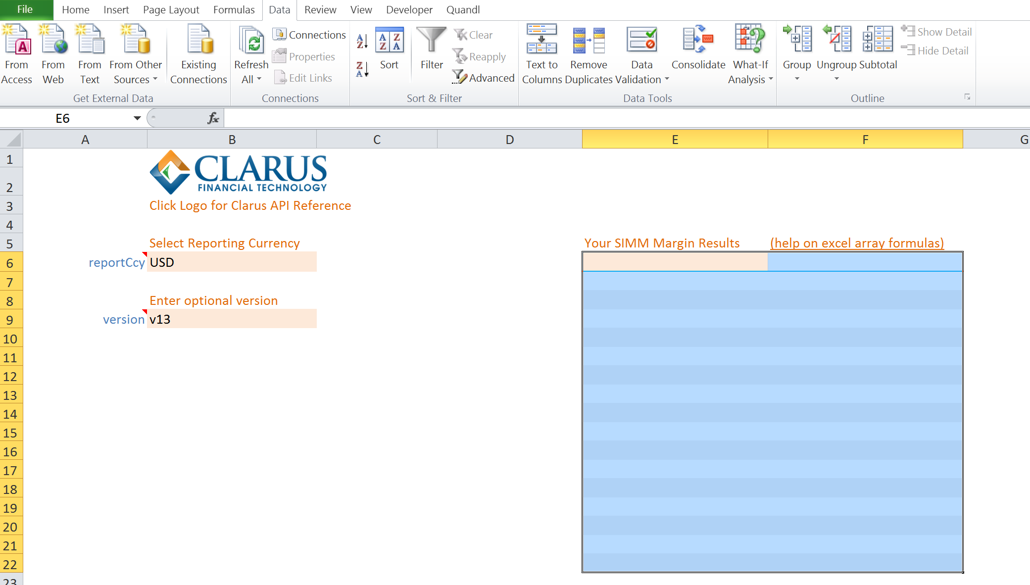
- Select the area on your spreadsheet that you want to return the data to.
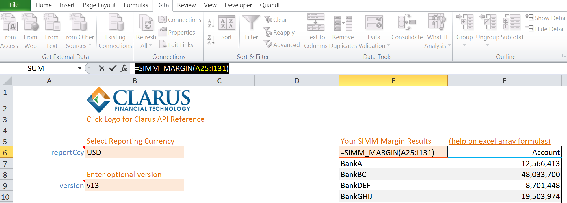
- Type in your formula, e.g. SIMM_MARGIN(<Range of Data>).
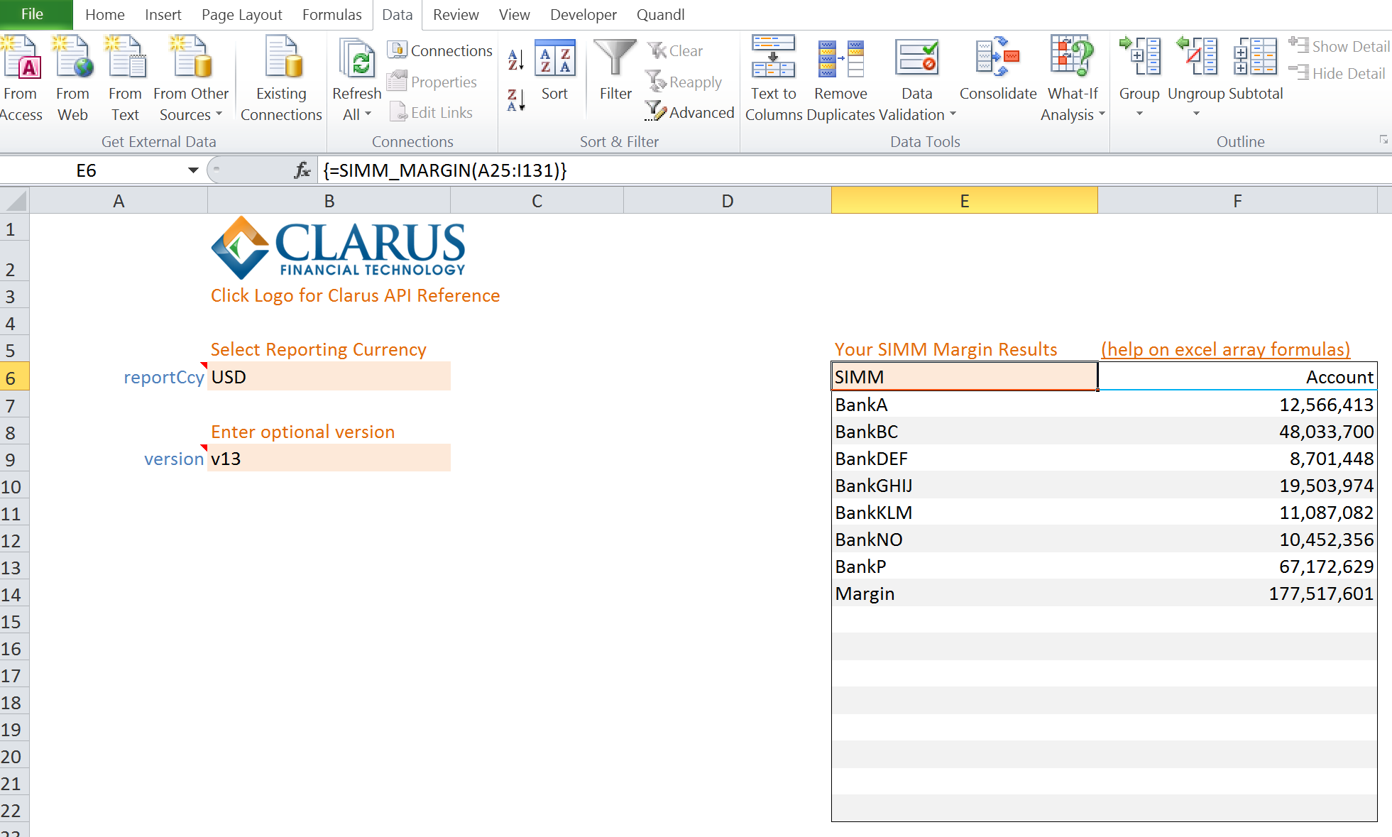
- Press CTRL+SHIFT+ENTER to confirm this formula (instead of just pressing ENTER). This will produce curly brackets {} around the formula. These curly brackets are how Excel recognises an array formula. They cannot be entered manually, they must be produced by pressing CTRL+SHIFT+ENTER.
We refer to CTRL+SHIFT+ENTER as the “Three Finger Salute”.
Working with Array Formulas
Array formulas act a little bit differently to other Excel formulas. Here are some things to remember:
Entering an Array Formula
- Remember to enter your formulas using the Three Finger Salute CTRL+SHIFT+ENTER.
Deleting an Array Formula
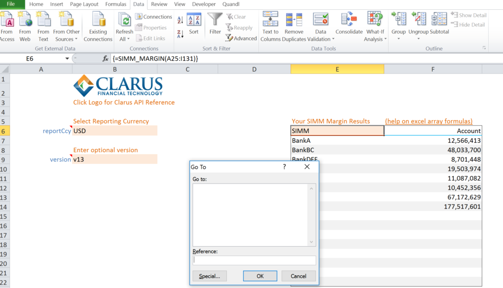
- To delete an array formula you must highlight the entire area of the spreadsheet where the array is entered. CTRL+/ is the quickest way to do this.
Editing
- The array formula itself always resides in the top left hand corner of the range. This is the only cell within the range that can be edited. The array formula will appear in all other cells of the range, but it cannot be edited in any cell other than the top left hand corner of the range.
Resizing
- To expand the range that an array formula writes to, start with the formula in the top left hand corner. Select the expanded range that you want to write to. Press F2 to edit the formula. Then use the Three Finger Salute to confirm the new, larger array.
- To shrink the range that an array formula writes to, you will have to delete the whole of the original range (CTRL+/ to select). Then select the new, smaller range, and re-enter the formula. This is less onerous if you copy the existing formula as a text string first (select in the formula bar and use CTRL+C):
Formatting
- Take the time to help yourself out. Format array areas in your spreadsheet consistently to provide a visual cue as to where your array formulas are. We also choose to highlight the top left hand cell of an array.
Get Used to Pop-Ups
- Even the most advanced and careful Excel wizards will occasionally forget that they are in an array. This happens to the best of us! Luckily, noting really bad happens, but you need to get used to the frustrating pop-up:
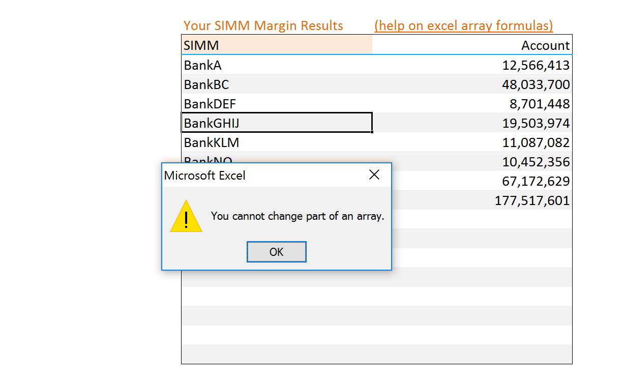
I always think “no it’s not okay Microsoft, that is really frustrating” so prefer to hit Escape to exit this message.
Tips and Tricks
Here are four shortcuts that I find amazingly useful when using spreadsheets with array formulas:
1. CTRL + /
This selects the current array. It is the shortcut for F5>Special>Current Array shown below: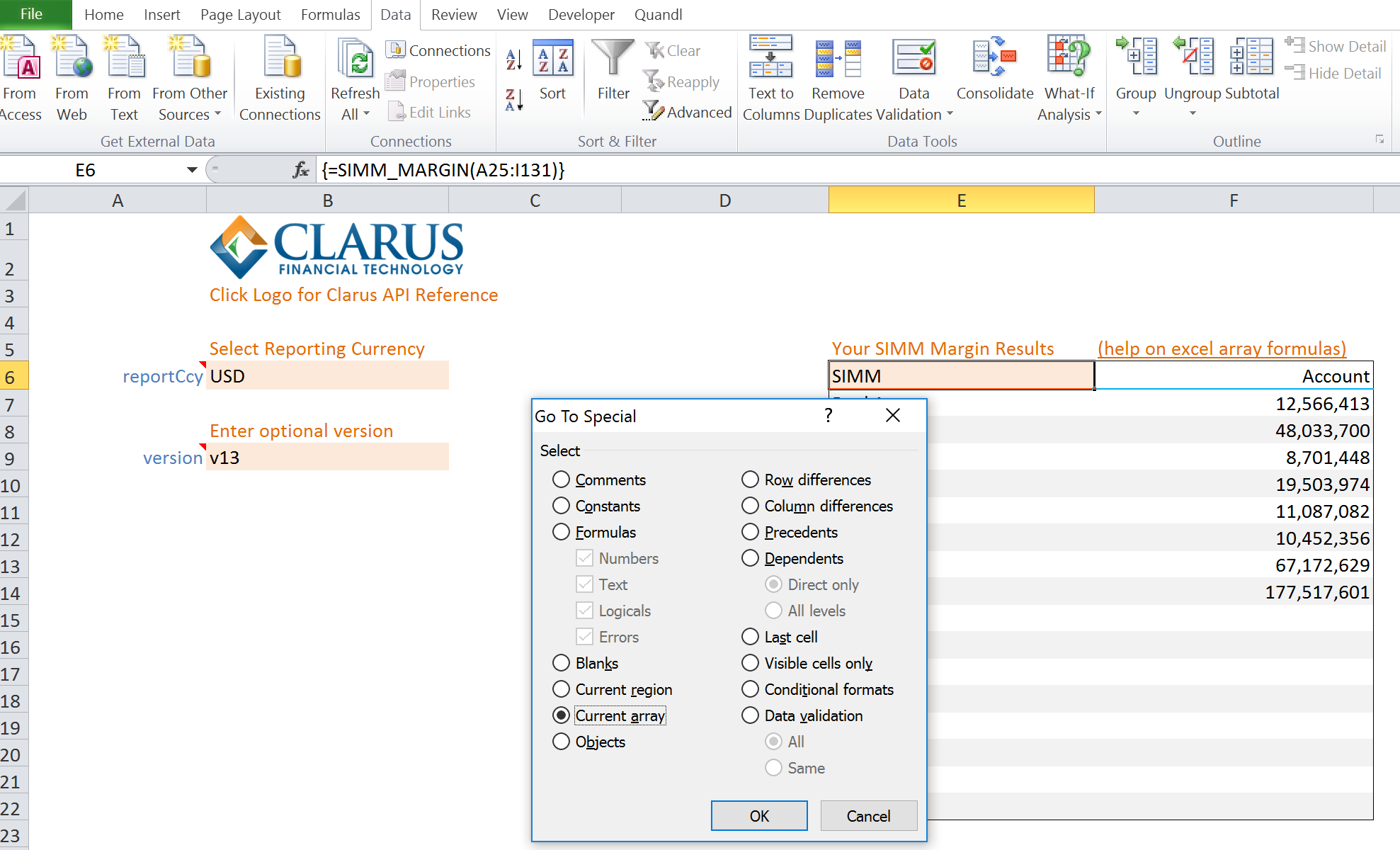
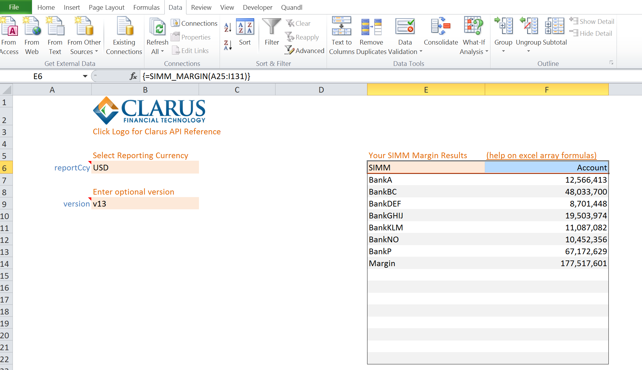
2. CTRL+SHIFT+RIGHT
CTRL+SHIFT+RIGHT highlights the current array to the right.
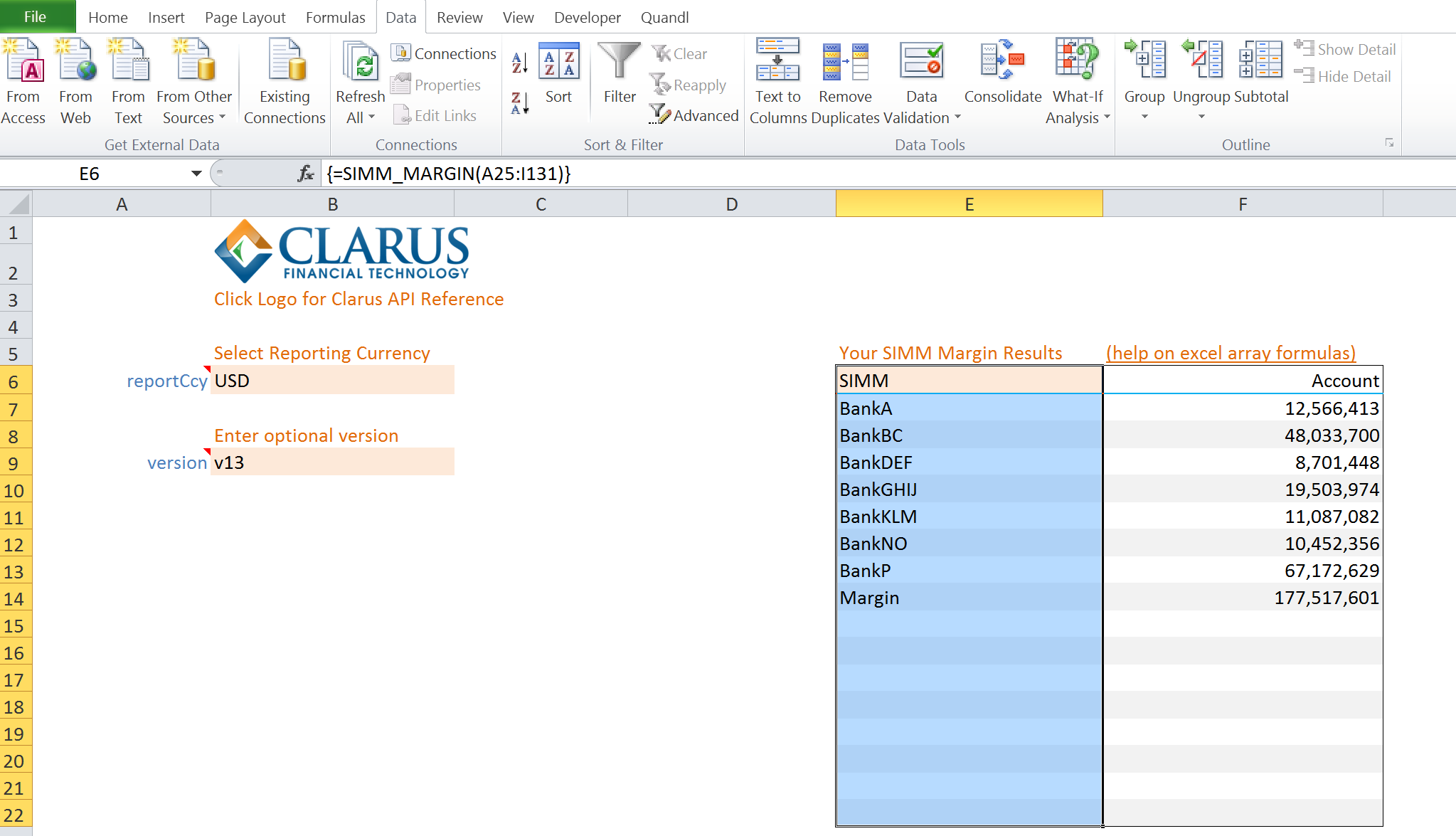
3. CTRL+SHIFT+DOWN.
CTRL+SHIFT+DOWN highlights the current array to the bottom.
4. F2 to Edit, Three Finger Salute to confirm
There is no need to select the whole of the array area if you want to edit the formula. Edit the top left hand cell by pressing F2, then confirm using the Three Finger Salute (CTRL+SHIFT+ENTER). This will automatically update the rest of the array.
In Summary
- Master the Three Finger Salute (CTRL+SHIFT+ENTER).
- CTRL + / is your friend.
- If you are unsure how large your data return will be, enter the array in a small area first. It is easier to expand arrays than shrink them.