SEF Packages, Swap Curve trades, do we need a new zero?

Motivated by the May 1, 2014 CFTC announcement on the ending of the SEF Package exemption, I decided to look at the package transactions that will shortly be mandatory to trade on a SEF.

For May16 these are packages where each component is a Swap that is MAT and for June 2 where one component is a Swap that is MAT and the other a Swap subject to mandatory clearing.

This means three commonly traded packages; Swap Curve, Swap Butterfly and Unwind/Offset packages.  In this article I will look at the Swap Curve and Swap Butterfly.

In particular whether the potential profits from these trades out-weigh the costs to such an extent that we can treat the costs as zero. Or whether the costs are significant enough that we need to define a new zero?

 

Swap Curve

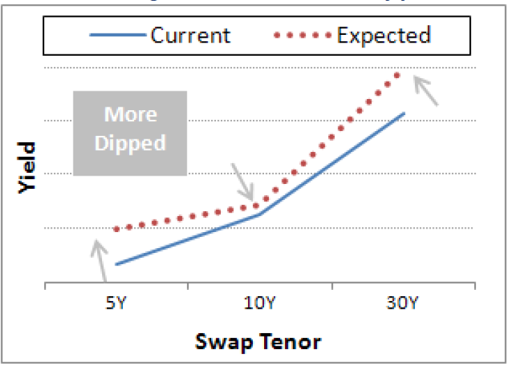
The Swap Curve  has two legs each of a different tenor and opposite direction (pay & rec) with notionals chosen such that the DV01 (change in value for a 1bps change in the rate) of each leg cancels the other.

Consequently the value of this trade does not change if the Swap curve moves in a parallel manner.

They are designed to make money when the Swap Curve Flattens or Steepens.

We know from principal component analysis that approximately 80% of a Swap curves change can be explained by the parallel shift factor. While 15% can be explained by a slope factor and 5% by a shape or curvature factor.

Swap Curve trades make or lose money depending on the slope factor.

An example trade would be a 5Y 10Y Swap Curve, where we pay fixed for 5Y on 260M notional and receive fixed for 10Y on 142m notional. This trade has a DV01 on each leg of $125,000, which net to zero.

 

Swap Butterfly

The Swap Butterfly has three legs of different tenor, with the middle leg notional (DV01) being equal and opposite to the sum of the two ‘wings’ DV01s.

Swap Butterfly trades make money when the swap rate of the middle leg changes more or less than the rates of the wings. That is the shape or curvature of the Swap curve changes. So if our expectation is that this will happen, we could trade this to make money.

(Picture Attribution: Swap Rate Curve Strategies, CME Group)

An example trade would be 5Y/10Y/30Y, where we receive fixed 10Y on 570M (DV01 is $500,000) and the 5Y and 30Y legs each have half the DV01 of the 10Y.

 

Credit Limit Checking

A quick diversion before we look at cost.

We know that some SEFs, CreditHubs, FCMs and CCPs have been using DV01, either gross or net in the acceptance process and doing so at a single swap level.

Well the Net DV01 check is not going to work as by definition Curves and Butterflys have zero DV01 and so would be accepted as risk-less! The Gross Dv01 is most likely going to reject such trades due to their large notionals.

I expect a lot of folks have been working to solve this and now the clock is about to run down. No doubt we will see some creative methods applied.

The correct method is to perform the credit acceptance check on incremental portfolio margin.

See my article on Push, Ping and Charm for details.

 

What are the Costs?

Lets start by distinguishing between one-time costs and periodic (daily/weekly/monthly) costs.

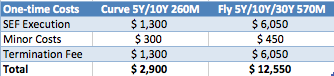
One-time costs:

1. SEF Execution fee to enter into the trade.
2. Minor costs – MarkitWire fee, SDR Reporting Fee and Clearing Fees.
3. Termination Fee to exit the trade.

Periodic Costs:

1. Funding Initial Margin.
2. Funding Default Fund Contributions (if applicable)
3. Funding Capital requirement.
4. Funding liquidity to meet daily variation margin.

 

One-time costs

SEF Execution fees (brokerage) is around 0.02 basis points per tenor year.

And for Swap Curve and Butterfly are charged on the gap in the tenors.

Ignoring any volume discounts, we can calculate these for our example trades.

(In the first version of this blog, I did not know that brokerage is present valued, which for these tenors is significant. Thank you to Tradition for pointing this out. I have now corrected the tables below).

We can also assume that termination fees are similar to execution fees on the assumption that rather than terminate we could put on the exit trade. In reality termination fees may be a higher as the tenors will no-longer be on the run.

All the other fees are flat fees, so not notional dependant.

For want of a better estimate let us assume $150 for all these, charged per swap leg.

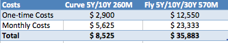
Our table of costs is then:

(Any remaining mistakes in the above are all mine and I would welcome any corrections).

 

Initial Margin

Before we look at periodic costs such as funding the Initial Margin, we need to know what the Initial Margin requirement is for these trades.

We can do this with CHARM and the below screen shots show this assuming CME is selected as the CCP.

Let start with the Swap Curve trade.

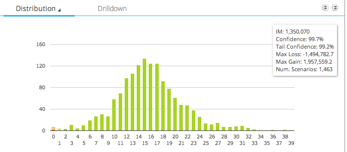
This shows us:

• A histogram of the profit and loss returns of this trade
• With most outcomes around zero
• The Initial Margin is $1.35 million
• We can also see the Max Loss and Max Gain (in this 5Y historical period of 5 day returns)
• Which are -$1.5 million and +$1.9 million

 

Lets now do the same for the Swap Butterfly.

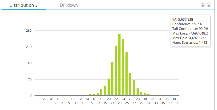
This shows us:

• A histogram of the profit and loss returns of this trade
• Again most outcomes around zero
• But this time the distribution has a much longer tail
• The Initial Margin is $5.6 million
• Max Loss is -$7.6 million
• Max Gain is $4.7 million

CHARM allows us to drill-down to explain these numbers.

However that is a blog for another day  or if you cannot wait, please contact us for details.

 

Periodic costs

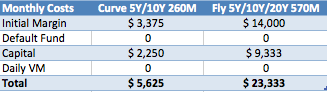
The first of these is funding the initial margin that is required by the Clearing House, in the form of cash or government securities.

It comes down to our costs of funds, which varies for types of financial firms. Lets assume we fund by raising debt and are able to issue this at 3.5%. Further that the CCP pays us 0.5% on our initial margin. We then have a net funding cost of 3%.

For our Swap Curve IM of $1.35 million, this is equal to $3,375 per month.

Contributions to Default Funds are required for Clearing Members, so lets cheat and assume we are a client and somehow not being charged something to cover this by our friendly FCM, who is keen to get our business.

Basle III requires 20% capital risk weighting for funds deposited at a CCP. Lets assume this is Tier 1 Equity Capital, which is much more costly than debt. Lets assume 10% and that only the IM is on deposit (so no Default Fund contribution and Variation Margin balance is zero). With these we can estimate the funding cost of capital.

(Correction: Jon Skinner commented that Default Fund contributions are very significant and need to be included for self-clearing firms,. And that while Basell regulatory capital is not typically charged to business lines but used as a return metric, Economic capital is though its calculation may different from the regulatory one. These are topics for another day).

Maintaining liquidity to meet the daily cash calls for variation margin is a trickier proposition to estimate. This need for cash might be met by the working capital and cash-flow of the business, for simplicities sake lets assume we are not charged for this.

(Correction: Jon also pointed out that the daily vm  cost is already factored into the pricing as daily margin in the currency of the trade and price alignment interest is assumed, so it is correct to treat as zero or in-fact not have in the table at all).

Lets now create a table of monthly costs.

(Again all mistakes are mine and I would appreciate any comments on the assumptions and calculations).

 

What are the Profits?

A reasonable question to ask is what are the potential profits from this strategy.

One indicator we have is the Initial margin itself. However we are not expecting to hold this strategy for 5 years in the expectation of one of those tail-gain scenarios happening again.

A more realistic horizon might be 1-month.

Using the past 6 months of data, we can look for what the returns from such trades would be. While the majority would be close to zero, we know that if the 1-month change in 5Y, 10Y, 30Y relative to each other is significant then our trades will show significant profit & loss.

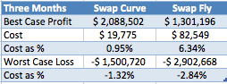
The table below presents eight such periods.

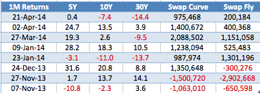
So had we timed our trades perfectly on 21 Mar, it would make us $975k on the Curve and $200k on the Fly, due to the 5Y increasing 0.4 bps, the 10Y dropping 7.4 bps and the 30Y dropping 14.4 bps in the month up to 21 Apr.

The largest gains are the 27 Mar scenario ($2m and $1.1) and the largest losses on the 27 Nov scenario ($1.5m and $2.9m).

So we can see that provided we can hold this strategy their is the opportunity for large profits or large losses.

 

Profits and Costs

Lets now bring together the costs and profits, starting with a table assuming that we put on these trades for one month.

We know that most of the time, holding this trade for a 1-month period will generate little or no profit. Recall our 80% parallel change factor. However we know that the other 20% will lead to meaningful profit & loss.

Lets assume that based on the last 6 months of data, we can time our trades perfectly to make the most profit or imperfectly to make the most loss. We can then create the following table.

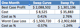
From which we can see that our cost expressed as a percentage of profit & loss is 0.4% or higher in each case.

If we were to hold these trades for 3 months (waiting for that gain) we would not generally expect a higher or lower loss, but we would increase the probability of either happening. However we know our costs would definitely be higher by monthly costs times two.

In this case the Butterfly trade costs start to look more expensive relative to its profit potential than the Curve.

This is due to the short six months of history that I have used to look for significant scenarios, which if we recall are change in shape factors (<5%). In addition the higher IM requirement for the Butterfly is driven by extreme tail scenarios from Oct 2008 (familiar?), while for the Curve they are not driven by these events.

 

Summary

Swap Curve and Swap Butterfly are Packages that will be mandatory to execute on a SEF after 15-May.

Swap Curve is designed to make money from changes in the curve slope (steepen or flatten).

Swap Butterfly from changes in the curve shape.

The costs to enter, maintain and exit these trades can be calculated.

The assumption that the cost of such trades are close to zero is no longer a good one.

In particular clearing requires funding the initial margin, which is significant cost and larger than the execution cost.

The more interest rates rise, the higher the costs of funds and the higher the cost of funding the margin.

The longer we hold the position, the more these costs become material but the more we increase our chance of large profits.