In a recent paper, “Calculating Delta Risks and Hedges via Waves (2015)“, Hagan deals with an old practical problem–determining risk and hedges on an interest rate book. In older systems a delta hedge report is often implemented by perturbing quotes used to construct the yield curves, restripping the curves and then revaluing the book. As curve construction became more sophisticated, and in particular, with the use of smooth global interpolators, this method produced some nasty side effects, most notably hedge leakage (or risk bleeding). To solve this problem some teams actually use a separate set of curves that rely on local interpolators so as to avoid the problem. The method of `waves’ suggested by Hagan is well-known to some practitioners for many years, but it is the first time I have seen a published paper dedicated to the topic. The methodology has several prominent virtues;
1. No hedge leakage,
2. Works directly on (smooth) pricing curves,
3. Flexibility – separated from the curve stripping algorithm and instruments.
Waves method can be described in several steps;
1. Specify a set of non-overlapping box-shift scenarios to the instantaneous forward curve,
2. Specify a set of spot starting swaps to act as hedges to the portfolio,
3. Compute the book’s sensitivity to each scenario,
4. Compute the hedging instruments’ sensitivity to each scenario,
5. Determine the size of the hedging instruments that match the portfolio’s risk under each scenario.
In short, the method determines a set of spot starting swaps whose risk is equivalent to the portfolio.
Forward Shifts
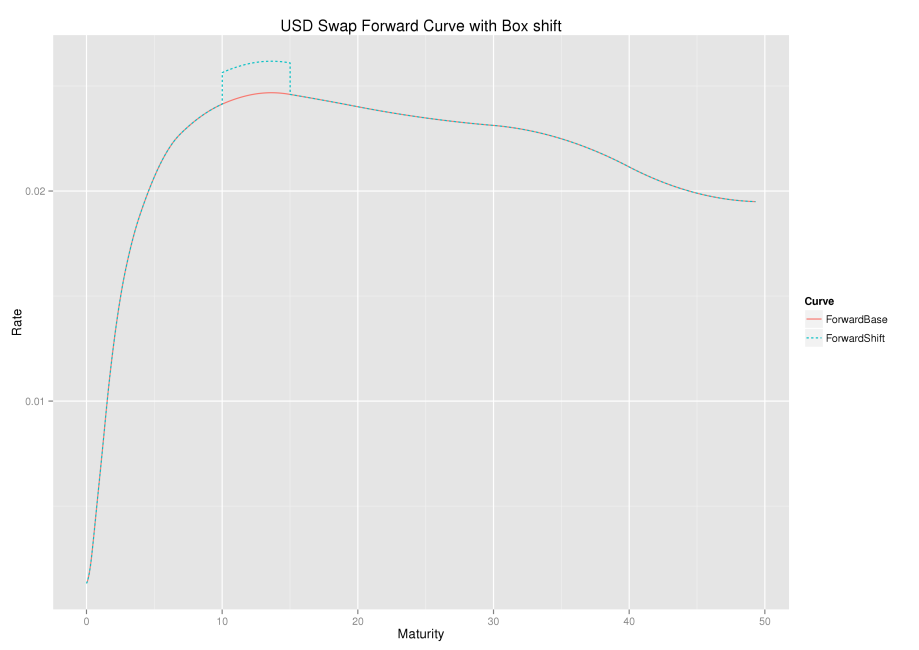
The idea of a box-shift on the instantaneous forward curve can feel slightly unusual to those more familiar with pointwise perturbation of input quotes or zero rates. The easiest way to think of the instantaneous forward rate curve, is to think of the curve consisting of 1-day forward rates as an approximation, and the box-shift is bumping a set of those rates between two dates. Hagan defines a sequence of non-overlapping box-shifts which cover the entire curve, the \(k^{th}\) shift being defined as
$$f_k(t)=f(t)+\delta \begin{cases} 0 & t < T_{k-1}\\ 1 & T_{k-1} < t < T_k \\ 0 & T_k < t\end{cases}$$.
An example is shown below.
The same base and shifted curve expressed in zero rates is shown below.
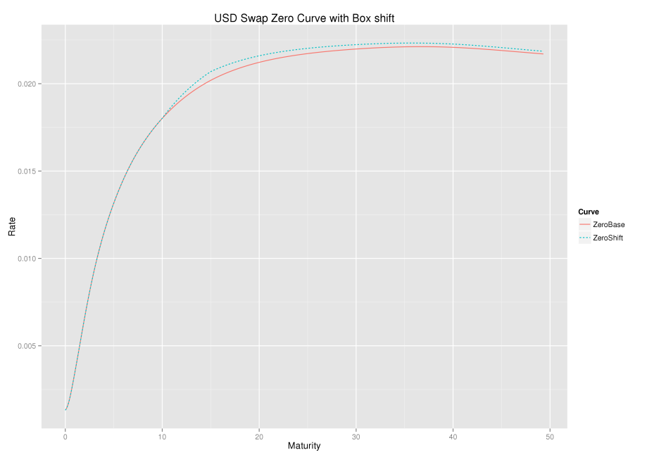
An alternative representation of the shifted curve is,
$$D_k(t)=D(t)\begin{cases} 1 & t < T_{k-1}\\ \exp(-\delta(t-T_{k-1}) & T_{k-1} < t < T_k \\ \exp(-\delta(T_k-T_{k-1}) & T_k < t\end{cases}$$
This representation can be of more practical value as most curves, regardless of their inner workings, will likely have an accessible discount factor function \(D(t)\).
From both representations and the associated graphs, one can see that a forward rate is only affected by a box-shift if the forward start or end date overlaps with the box shift start and end date. Further, any discount factor is affected by the shift if its payment date is after the box shift start date.
The Wave
The chart below shows a set of box-shifts being applied one at a time; the box-shift ripples along the forward curve.
Linear Algebra
In Hagan’s paper, the scenarios and hedge instruments inextricably linked; the box shifts are defined by end dates of the hedging instruments. In this case, the determination of the size of the hedge instruments is the solution to a classic linear algebra problem of the form $$Ax=b$$
Whilst this problem appears in the recent Wilmott magazine article, it is also sketched in the 2006 paper by Hagan and West, Interpolation Methods for Curve Construction.
One might naturally seek a smaller subset of instruments, but retain the granularity in the scenarios (and hence the portfolio’s risk measurement), in which case, there is unlikely to be an exact solution. Instead one can choose hedge sizes which most closely match the portfolio’s risk, in the least squares sense; that is, minimise $$||Ax-b||^2$$ The solution can be found by computing the pseudo-inverse (Moore-Penrose) of \(A\). In both cases, the problem formed makes no attempt to control the size of the hedge, the focus is only on closely matching the portfolio’s risk. More control over the hedge sizes can be found using ridge-regression or Tychonoff regularisation, where one is minimising
$$||Ax-b||^2 + \lambda ||x||^2$$
This approach is suggested by Lesniewski in his 2007 course notes, and again in his 2010 course notes.
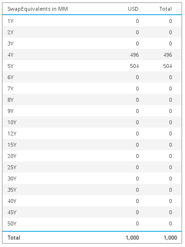
Multi-Currency Swap Equivalents View
Pulling all of the steps together allows us to construct a flexible and consistent view of portfolio risk expressed in swap equivalents across multiple currencies in CHARM.
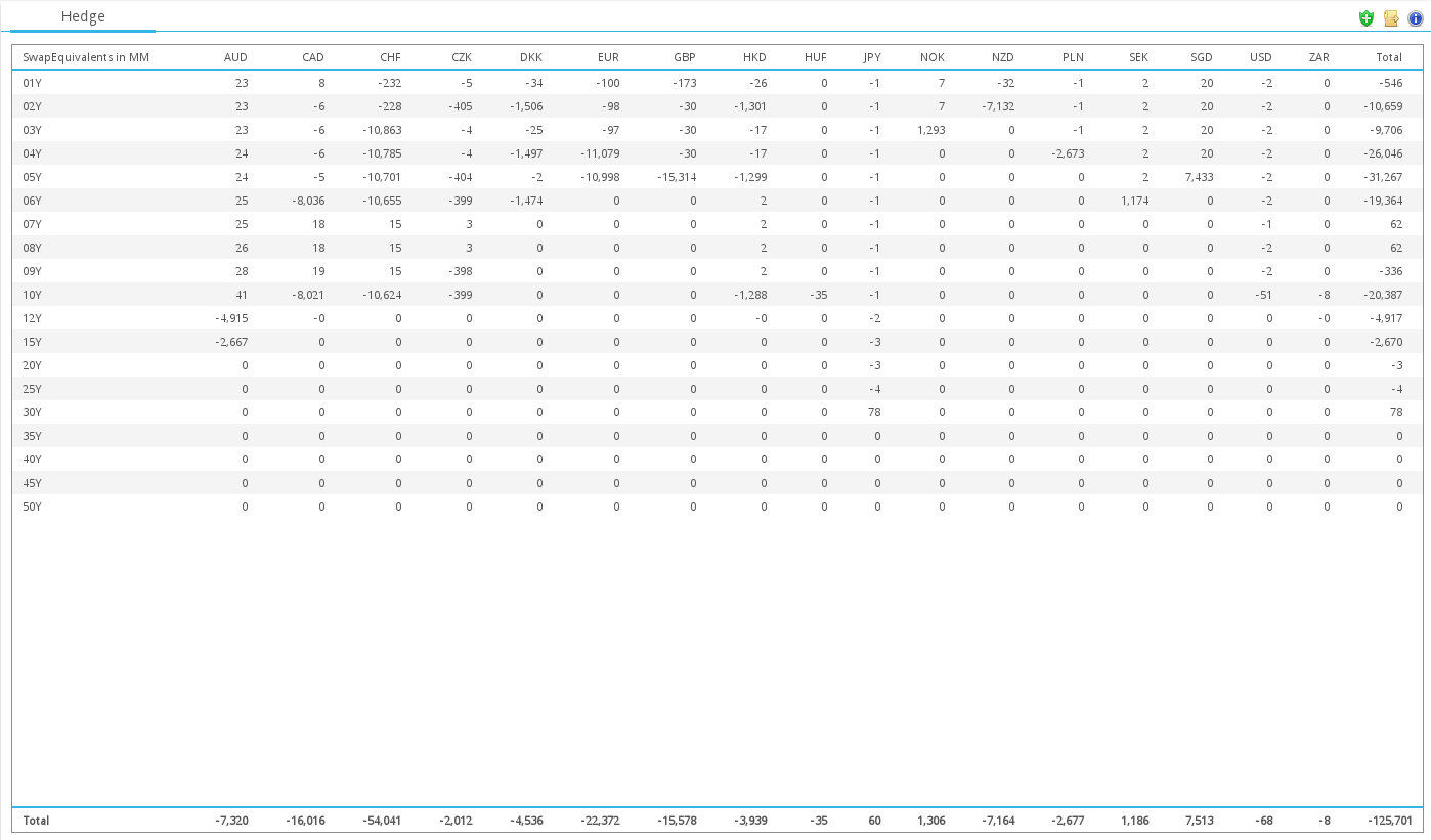
No hedge leakage
A quick test to check for hedge leakage is to consider a 4.5 year swap, we expect the equivalent swap risk to appear at the 4 and 5 year buckets.
Conclusion
Hagan’s wave method is a simple yet powerful addition to a risk system.
Box-shifts of the forward rate curve are used to express portfolio risk.
Known problems when using modern curve building routines in risk analytics are alleviated.
A separate set of simple risk curves are not needed, original pricing curves can be used directly.
A systematic consolidated view of risk across many currencies in terms of intuitive swap equivalents is possible.