 Using Java I implemented the double precision algorithm to compute the cumulative bivariate normal distribution found in A.Genz, “Numerical computation of rectangular bivariate and trivariate normal and t probabilities”, Statistics and Computing, 14, (3), 2004.
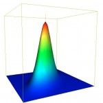
$$M(a,b, \rho)=\frac{1}{2\pi\sqrt{1-\rho^2}}\int_{-\infty}^a\int_{-\infty}^b \exp\left(-\frac{x^2-2\rho xy +y^2}{2(1-\rho^2)}\right)dxdy$$
To validate the implementation I had hoped to find an easily accessible table of values to check against, alas even my trusted copy of Abramowitz and Stegun: Handbook of Mathematical Functions did not have tablulated values, so I considered alternatives. Firstly, I considered the analytic result
$$M(0,0,\rho)=\frac{1}{4}+\frac{\arcsin(\rho)}{2\pi}$$
which leads quite naturally to the simple test values
| \(\rho\) | \(M(0,0,\rho)\) |
|---|---|
| \(0\) | \(1/4\) |
| \(1/2\) | \(1/3\) |
| \(-1/2\) | \(1/6\) |
| \(1/\sqrt{2}\) | \(3/8\) |
| \(-1/\sqrt{2}\) | \(1/8\) |
| \(\sqrt{3}/2\) | \(5/12\) |
| \(-\sqrt{3}/2\) | \(1/12\) |
| \(1\) | \(1/2\) |
| \(-1\) | \(0\) |
Elegant as they are, these special cases only cover only a small part of the algorithm, however randomly picking \(\rho\in(-1,1)\) and comparing to a computed value of \(1/4+\arcsin(\rho)/2\pi\), covers much of the code and is quite accessible since a double precision implementation of \(\arcsin\) is available in most languages.
Finally, I generated values from the statistical package R (library mvtnorm) at specific points which ensure 100% coverage of the algorithm.
| \(a\) | \(b\) | \(\rho\) | \(M(a,b,\rho) \) |
|---|---|---|---|
| \(0.5 \) | \(0.5 \) | \(0.95 \) | \(6.469071953667896E-01\) |
| \(0.5 \) | \(0.5 \) | \(-0.95 \) | \(3.829520842043984E-01\) |
| \(0.5 \) | \(0.5 \) | \(0.7 \) | \(5.805266392700936E-01\) |
| \(0.5 \) | \(0.5 \) | \(-0.7 \) | \(3.98076964063486E-01\) |
| \(0.5 \) | \(0.5 \) | \(0.2 \) | \(5.036399310969482E-01\) |
| \(0.5 \) | \(0.5 \) | \(-0.2 \) | \(4.538723806509604E-01\) |
| \(0.5 \) | \(0.5 \) | \(0.0 \) | \(4.781203353511161E-01\) |
| \(-0.5 \) | \(0.5 \) | \(0.95 \) | \(3.085103770696148E-01\) |
| \(-0.5 \) | \(0.5 \) | \(-0.95 \) | \(4.455526590722349E-02\) |
| \(-0.5 \) | \(0.5 \) | \(0.7 \) | \(2.933854972105271E-01\) |
| \(-0.5 \) | \(0.5 \) | \(-0.7 \) | \(1.109358220039195E-01\) |
| \(-0.5 \) | \(0.5 \) | \(0.2 \) | \(2.375900806230527E-01\) |
| \(-0.5 \) | \(0.5 \) | \(-0.2 \) | \(1.878225301770649E-01\) |
| \(10.1 \) | \(-10.0 \) | \(0.93 \) | \(7.619853024160583E-24\) |
| \(2.0 \) | \(-2.0 \) | \(1.0 \) | \(2.275013194817922E-02\) |
There is a table of computed values in Haug’s book, “The complete guide to option pricing formulas“, Second Edition, however it has only one value in the interesting area \(|\rho| \in(0.925,1)\), and that test value is an extreme.
Yes I either use R or Scilab to validate algorithms. Both together have a good coverage of math stuff. Scilab code is not too bad either, it’s often interesting to look at their method signatures.
There is a table of value for the Cumulative Bivariate Function in Haug p481
Already looked at Haug’s table, there are no interesting cases for \(|\rho| \in (0.925,1)\).
It would have been interesting to know why you needed the distribution function. Is it for double barriers?
The first time I needed to use cumulative bivariate (and trivariate) normals, was for window barrier options in FX, specifically the paper by Grant Armstrong, “Valuation formulae for window barrier option”, Applied Math Finance, 2001. Quite an interesting paper is by Graeme West, “Better approximations to cumulative normal functions”, which highlighted some problems with popular approximations in finance before Genz. The bivariate normal appears in the theoretical valuation of compound options and American option approximation of Bjerksund and Stensland, as well as partial barrier options.
For this implementation and tests there is a pull request on OpenGamma’s github repo.
Thanks. Surprisingly, the Quantlib code credits Graeme West, but actually is a port of Genz code. West suggests the use of DW2 algorithm, which looks quite different. Vasicek has also written some numerical implementation based on a different series expansion that is supposed to be more efficient when the correlation is > 0.5.
Graeme had C++ source code associated with his paper on his website http://www.finmod.co.za/research.html which included a C++ port of the Genz algorithm with some convenient modifications for finance, that is probably why Graeme’s paper is referenced. This actually confused me when looking at OpenGamma implementation, the documentation mention Graeme’s paper but the algorithm was not the Genz algorithm that I was familiar with because of Graeme’s paper.