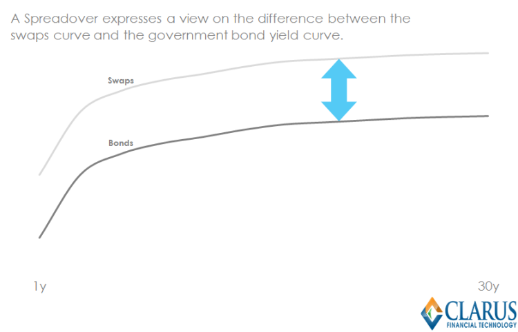
We define the characteristics and mechanics of a Spreadover or Swap Spread (“U.S. Dollar Swap Spread” in CFTC parlance). The inclusion of Spreadovers in our SDR products allows us to look at the volume of Swaps that are traded as a spread to Government Bonds.
Spreadover Definition
Trading strategy; to take a view on the difference in rates between an Interest Rate Swap and a Government Bond.
Any interest rate swap will make or lose money as rates go up or down. But what if an investor does not have an opinion on whether rates will go up or down? Perhaps, they think that the credit-worthiness of the financial industry will change relative to sovereign debt? Maybe our investor thinks that markets are poised for a Flight to Quality, or that other investors want to avoid Libor-based instruments and the lack of liquidity in associated swaps. In this case, they can transact a Spreadover.
This strategy highlights a very important feature of Spreadover trading. These trading strategies rely on relative moves between two markets. In the case of a 10 year swap versus a 10 year bond, if interest rates on the two instruments moved exactly in tandem, then we would not make or lose money (assuming cost of carry and the shape of the curves are consistent across the two markets).
Mechanics of a Spreadover Trade
Price
Let \( S_{(0,t_1)} \) denote the Swap rate between \( t_0 \) and \( t_1 \); and \( B_{(0,t_1)} \) denote the Government Bond yield between \( t_0 \) and \( t_1 \); the Price, \(P_{(0,t_1)}\) of the Spreadover is expressed;
\(P_{(0,t_1)}=S_{(0,t_1)} – B_{(0,t_1)}\)
The price of a Spreadover trade is the yield spread between the two instruments, expressed in basis points. Because Interest Rate Swap rates are typically higher than Government Bond yields (a.k.a the credit premium), it is conventional to quote a spread as a positive number and calculate the price as the Interest Rate Swap rate minus the Government Bond yield. This isn’t to say that Spreadover rates cannot go negative. Interest Rate Swaps are collateralised (and cleared versus a CCP), therefore an Interest Rate Swap may be perceived as being less of a credit risk than Government Bonds.
Size
Let \( DS_{(0,t_1)} \) denote the DV01 of Swap \( S_{(0,t_1)} \) between \( t_0 \) and \( t_1 \); and \( DB_{(0,t_1)} \) denote the DV01 of Government Bond \( B_{(0,t_1)} \) between \( t_0 \) and \( t_1 \);
\(0=DS_{(0,t_1)} – DB_{(0,t_1)}\)
This relationship will hold when both products are traded at market. The degree of convexity on each instrument may be (very slightly) different, therefore the position may need to be rebalanced following particularly large market moves.
When trading a Spreadover, we may agree a notional amount of the bond, and calculate a notional amount for the swap accordingly (or vice versa). The sum of the two DV01s (the “delta”) will be zero, hence a Spreadover trade is considered “delta-neutral.”
Coupons
Let \( P_{(0,t_1)} \) denote the Spreadover price between \( 0 \) and \( t_1 \);
\( B_{(0,t_1)} + P_{(0,t_1)} = S_{(0,t_1)} \)
The Government Bond yield is set at prevailing market rates. Assuming the Spreadover is at market, this inherently means that the Net Present Value (NPV) of the Swap leg is zero.
Direction
We always talk in terms of the bond leg. Therefore, if the investor is buying (selling), paying (receiving), lifting (hitting), taking (giving) or putting on a widener (tightener) they are buying (selling) the Government Bond, and paying (receiving) on the Fixed leg of the swap.
Spreadovers in the data
The USD Swaps market is thankfully a simple beast. As such, the particular form of Spreadovers in US markets that trade the most are also one of the most simple.
We do not worry whether \(t_1\) for the Bond, \(B_{(0,t_1)}\), is exactly the same as \(t_1\) for the Swap, \(S_{(0,t_1)}\). So long as \(t_1\) ~\(t_1\) then we are happy enough. This is virtue of frequent refunding cycles of US Treasuries, such that the current On The Run (OTR) is always pretty close to its’ intended benchmark maturity.
Onto the data, and we see a significant volume of Spreadovers trading every day:
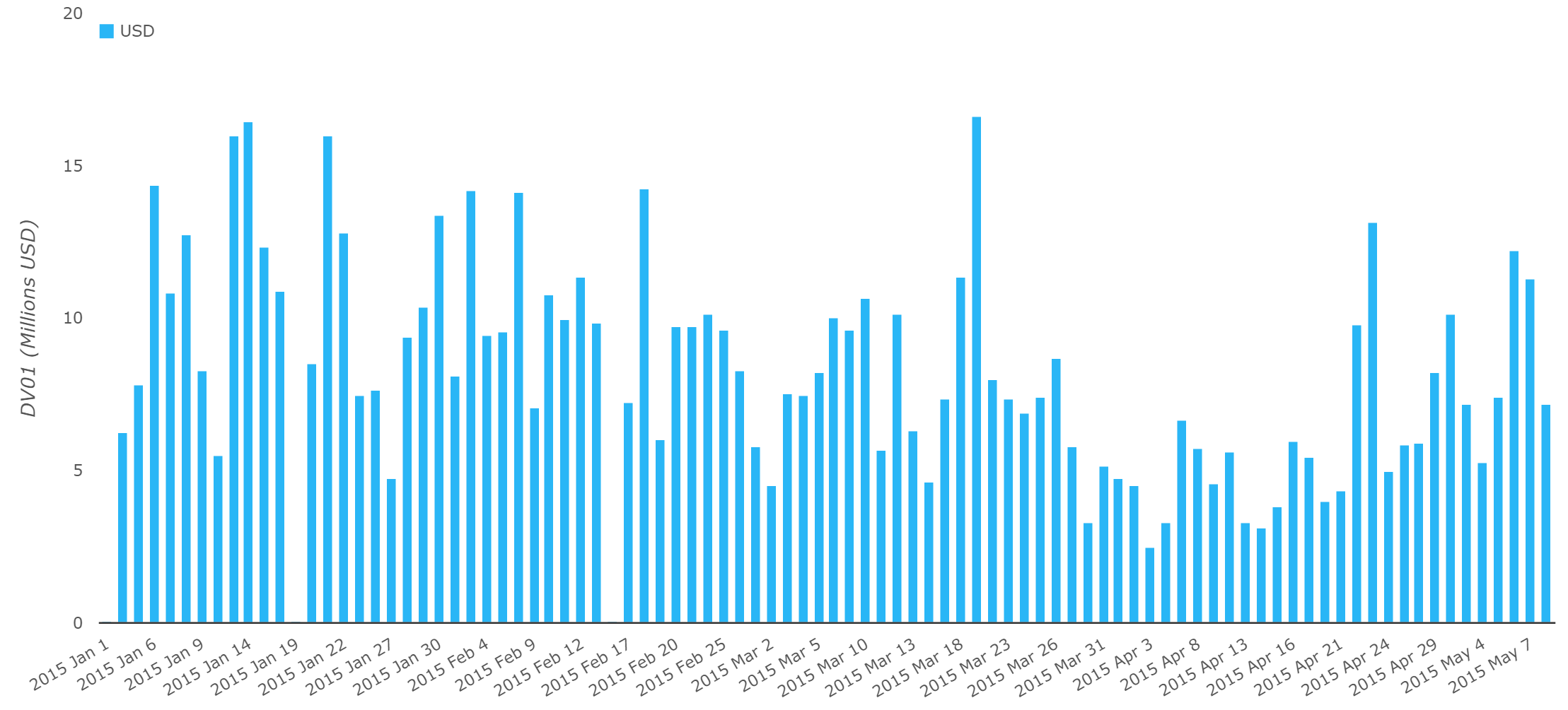
- On average, $8.1m in DV01 per day has traded in Spreadovers for 2015.
- Putting this into perspective, this accounts for around 15% of risk traded every day (excluding Compression and List trading).
- 19th March saw the largest amount of risk traded this year, at $16.7m DV01. This did not coincide with the same peak day for overall risk traded this year (which was 5th Feb).
- Wednesday and Thursday of last week saw unusually large volumes, but this was in-line with the spike in activity we saw in Swaps markets overall as a result of the extreme price volatility in underlying bond markets. If anything, it is surprising that Spreadover volumes were not higher.
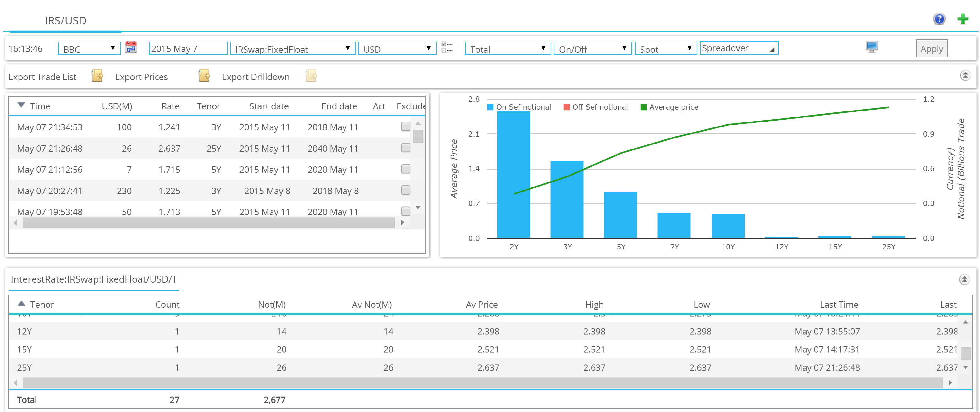
We can also use SDRView Pro to analyse the tenors that have been trading in notional terms:
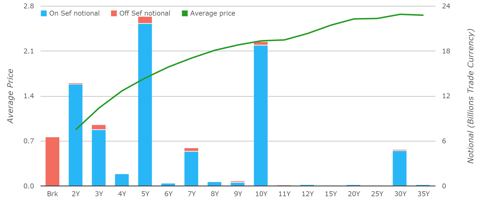
Showing:
- 5y (27%) and 10y (23%) have dominated trading during May 2015, with 2y,3y, 7y and 30y all recording significant volumes.
- 89% by notional have been executed on-SEF so far during May 2015, consistent with the mandate to trade Spreadovers on-SEF since June 15th 2014 (page 5).
SEF Market Share in Spreadovers
We can also use SDRView Res to look at the daily history in DV01 terms for BSEF. What we see is:
- An average daily market share of 12% during 2015 for Bloomberg in Spreadovers.
- There are end-of-month spikes, with the Bloomberg market share increasing above 20%.
- Overall, Bloomberg seem to have a lower market share of the Spreadover market (12%) than overall (~30%).
Stay tuned!
As I said, the USD Swaps market trades a very simple version of Spreadovers (also known as US Dollar Swap Spreads in CFTC parlance). Keep an eye out for a follow-up blog highlighting some of the other asset swap structures that are traded across other markets.