- What is the market risk capital charge for a bank trading an interest rate position?
- We calculate some examples using the Sensitivities-based Method under FRTB standards
- We find that a standalone 10y USD IRS results in a market risk capital charge of nearly 10% of the swap notional
Fundamental Review of the Trading Book
Following on from Amir’s look at FRTB and the different approaches available, I will dig into the numbers to expand on the Standardised Approach for Interest Rate Swaps.
Our reference document throughout is the BCBS January 2016 publication “Minimum Capital Requirements for Market Risk.” Having previously implemented the ISDA SIMM IM models in Excel, the similarities are striking for the Interest Rate portion of risk. It is worth bearing in mind that the ISDA SIMM documentation is written in a more logical order for the purposes of implementing the calculations.
Therefore, if you haven’t previously, I would take a look at ISDA SIMM in Excel if you are interested in replicating the calculations yourself.
I will follow the same format as my previous blog to explain the calculations below.
Sensitivities-based Method: Delta
To calculate the Market Risk under the Standardised Approach for an Interest Rate swap, it is important to take note of an incongruous paragraph at the very beginning of Section 4:
Meaning;
- As a trader, I am used to thinking of “Buckets” by maturity. e.g. if I trade a 2y vs 10y spread, I would be DV01 neutral across the curve, but with “bucket” risk in 2y and 10y.
- This is NOT what BCBS mean by buckets. I spent a lot of time going round in circles until I re-read this section about 6 times!
- So when looking at the Delta risk of your portfolio, please remember that when BCBS refer to a “bucket” they actually mean a “currency“.
- Almost any other word would have been better for my understanding here. Why not “risk-factor”, “currency”, “group”, “category”, “classification”, “set”, “batch”, “type”, “variety”, “family”. You can choose your own synonym….
This bug-bear aside, once I figured this out, the computations are as straight-forward to follow as for ISDA SIMM – something Amir has touched upon in his previous blog, and hence why I will follow the same 5 steps as from my ISDA SIMM blog.
1. Risk
There are 10 risk vertices onto which we must project our Interest Rate delta. We are used to dealing with DV01s; FRTB uses DV01 multiplied by 10,000:
\( \tag {1} \LARGE s_{k,r_{t}} = \frac{V_{i}(r_{t} + 0.0001, cs_{t}) – V_{i}(r_{t},cs_{t})}{0.0001}\)Where;
- \( s_{k,r_{t}}\) is the FRTB Sensitivity
- \( V_{i} \) is the market value of the instrument
- The equation means that we are shifting \( V_{i} \) by 0.0001 (i.e. 0.01%) on the risk free curve, \(r_{t}\), whilst keeping the credit spread, \( cs_{t} \), constant.
- We then divide this DV01 by 0.0001 (i.e. we multiply by 10,000).
The 10,000 scalar appears to be so that Risk Weights (see next section) can be expressed in percentages rather than conventional units. Does this make it easier for non-Rates people to relate to the risk weights?
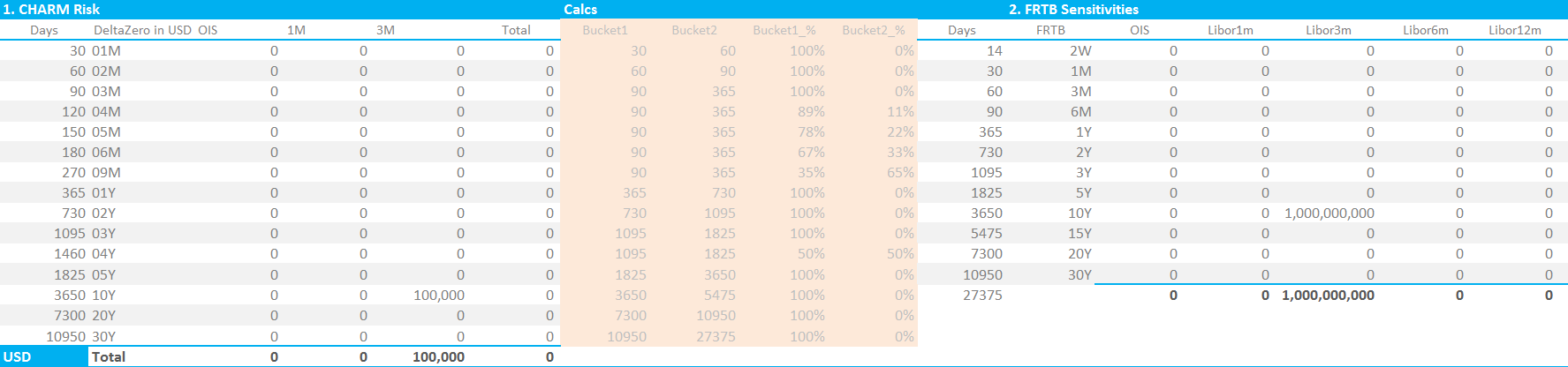
Showing;
- The DV01 analysis of a ten-year USD IRS from our risk analytics platform, CHARM, mapped onto the FRTB Risk Vertices
- This results in an FRTB Delta Sensitivity of $1bn.
2. Risk Weightings
The Risk Weightings that are applied to these Sensitivities vary by Risk Vertex as expected. Please note that the FRTB guidelines include the below table:
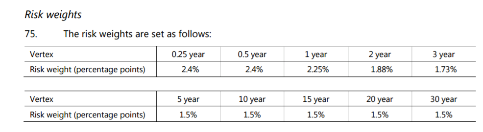
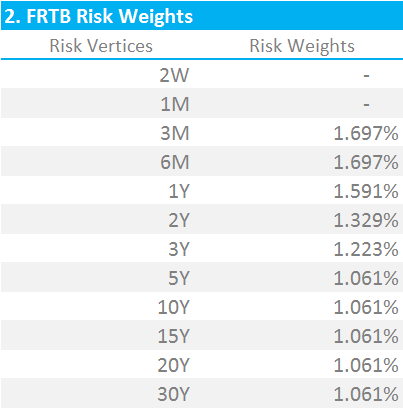
For the major currencies, we must divide these Risk Weightings by the square root of 2 (see table to the right). The BCBS committee have defined the major currencies as:
- EUR
- USD
- GBP
- AUD
- JPY
- SEK
- CAD
- Plus the bank’s designated domestic currency
At the end of this step, we end up with a “Weighted Sensitivity”, \( WS_{k} \) for each vertex. The next step explains how we aggregate these multiple “WS” values together.
3. Correlations
We must now use correlations between all of the Risk Vertices across different Indices within a single currency to decide how much offset we apply for any given position. For this, we turn to the familiar-looking formula:
\( \tag {2} \large K_{b} = \sqrt{\sum\limits_{k}{WS_{k}^2+{\sum\limits_{k}}{\sum\limits_{(k)≠(l)}ρ_{kl}WS_{k}WS_{l}}}}\)Where;
\( {WS_{k}}\) is the Sensitivity at a given tenor multiplied by the BCBS-supplied risk weighting.
\({ρ_{k,l}}\) represents the correlation of the “WS” terms from one tenor (“risk vertex”) to the next. These correlations must be calculated according to a BCBS-supplied formula and vary depending on whether we are comparing risk vertices on the same underlying index or across indices.
The formula to calculate the correlations to use looks a little daunting, but it is relatively trivial to implement;
\( \tag{3} \large max[e^{-θ.\frac{|T_{k}-T_{l}|}{min(T_{k};T_{l})}};40 \% ]\)Footnotes 25 and 26 in the BCBS document provide very useful worked examples to sanity check this implementation. The resulting correlation matrix is shown below:
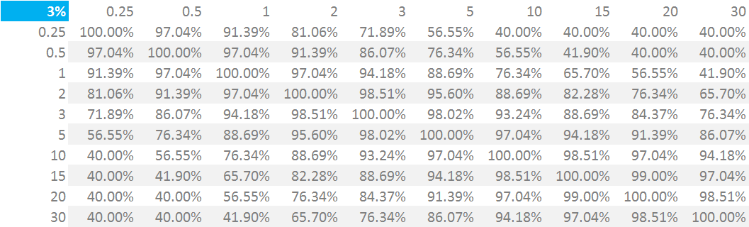
Showing;
- The correlations between tenor points for the same index. This I think of as the “within-index” correlation matrix. For example, a 10Y tenor is deemed to have a 76% correlation with the 1Y tenor.
- We also need to calculate the correlations between different points across different indices AND tenors. This I refer to as the “between-indices” correlation matrix. These correlations are calculated by multiplying the above correlations by a SubCurve correlation factor which is 99.9%.
- These correlations allow us to do two things. One is to combine a Weighted Sensitivity in e.g. the USD 3M Libor Risk Vertex with a WS in the 10y Risk Vertex of the same index.
- And secondly, combine a WS in the e.g. 1Y risk vertex of the USD 3M Libor index with a WS in the 10Y risk vertex of the USD OIS index.
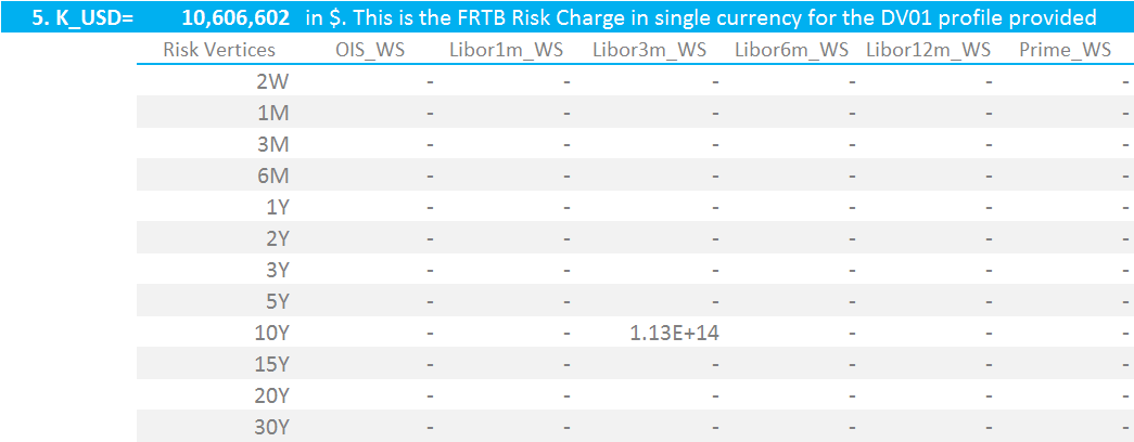
4. Calculate the FRTB Risk Charge
Armed with our matrices of WS terms and Correlation factors, we now simply multiply one matrix by the other, according to equation 2 above.
For a 10 year USD swap in $100,000 DV01, this results in the below matrix:
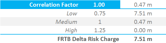
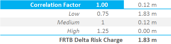
5. Run the Correlation scenarios
There is an additional provision in the FRTB guidelines to allow for the fact that correlations may change over time. Paragraph 54 states:
In order to address the risk that correlations increase or decrease in period of financial stress, three risk charge figures are to be calculated for each risk class
What this means is that we must vary the correlation coefficients. \(ρ_{kl}\) (correlations within the same currency) and \( γ_{bc}\) (which we haven’t introduced yet, but is the correlation between currencies) must be uniformly multiplied by 1.25, 1.0 and 0.75. The ultimate capital charge is the largest of the three results.
6. Sanity Check the Results
To check my model, I used the following test cases. These can easily be compared to ISDA SIMM (which remember is Initial Margin, NOT capital) by referring to my previous blog.
10y USD Swap in $100,000 DV01. Capital Charge = $10.6m

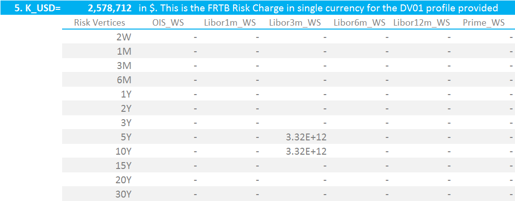
5y vs 10y USD 3m Libor swaps in $100,000 DV01. Capital Charge = $2.6m
USD 3m Libor vs USD OIS 10y Basis in $100,000 DV01. Capital Charge = $7.5m
A USD Box trade – 5y10y in OIS vs 3m Libor in $100,000 DV01. Capital Charge = $1.83m
A Quick Analysis
We will revisit these results in future blogs. However, from my first assessment, I notice that:
- These capital charges are higher than I expected. I have not looked in detail at the calibration process, but I expected figures similar to those from the ISDA SIMM calibration.
- A 5y vs 10y curve trade (example 2 above) creates a lower capital charge than a 10y OIS basis trade (example 3 above).
- This is because any interest rate trade incorporating a degree of “basis” – i.e. across different indices – must run three correlation scenarios, changing the coefficients by 25%.
- This has implications for complex portfolios that have risks across multiple indices and multiple currencies.
- These numbers will impact the decision to use the Standardised Approach versus obtaining model approval and applying the Internal Models Approach.
In Summary
- We work through the BCBS documentation to present initial findings on the Standardised Approach.
- Under this framework, a standalone 10y USD IRS in $100k DV01 creates over $10m in Capital Charges. This is equivalent to nearly 10% of the trade notional.
- Real-life bank portfolios will be more complex than this simple example.
- From our initial analysis, it is basis trades across more than one index that may prove to be costly from a capital perspective.