- We build an IM calculator in Excel for Equity Derivatives under ISDA SIMM™.
- The methodology builds on the margin methodology for Rates products, and uses very similar formulae.
- We cover all forms of IM. This blog is for the Delta Margin.
- There are subtle differences to the implementation for Rates, mainly around the concept of “buckets” of risk.
- UPDATE: We now offer free 14-day trials for our SIMM for Excel product
Equity Derivatives Initial Margin
So far we have successfully built and maintained Excel spreadsheets to calculate Delta IM for rates products, for multi-currency portfolios and also for Swaptions that cover both Vega and Curvature IM. Given the remit of ISDA SIMM™ to be easy to replicate, I thought this week I would turn my focus to an asset class I have little experience of – Equity Derivatives. The ISDA reference docs are here.
1. Risk Sensitivities For Delta
For Delta inputs, the sensitivities are much as we were with Rates. For Delta;
\( \tag {1} s = V(x+1 \%.x)-V(x)\)i.e. we bump the price of the underlying equity by 1% and record the valuation change (V).
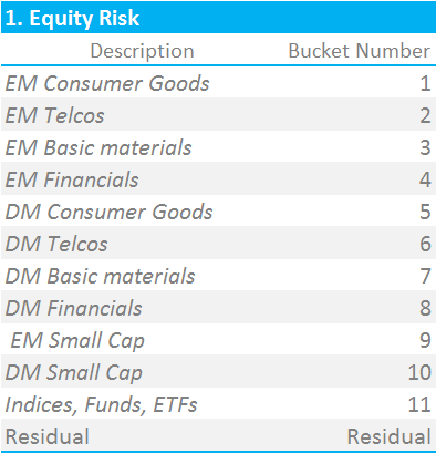
We must now assign each position to a Risk Bucket. There are 12 categories defined by ISDA as per the below:
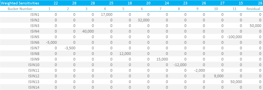
Below is a representative input grid of positions, mapped to their Risk Buckets:

Showing;
- Each security is mapped to only one “risk bucket”.
- The mapping is security specific, with ISDA providing guidelines on which bucket to map a given security to.
- Indices/ETF/Fund exposures are all in Bucket 11, which carries a substantially lower risk weighting than other buckets.
2. Risk Weightings
We now apply the requisite risk weights to each bucket, according to the ISDA calibration. This is a simple look-up table providing a Risk Weight per bucket:
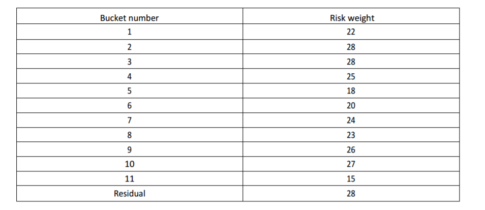
For now, I will run these assuming that we are below the Concentration Threshold. Please refer to my separate blog on Concentration Thresholds for the implementation of these risk multipliers.
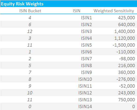
Showing;
- Each security is now mapped to the appropriate Risk Bucket and has a weighted sensitivity.
- It is important to note that identical securities within the same product class should have their positions netted together at this level.
- It is possible to have multiple securities mapped to the same Risk Bucket (e.g. I have both ISIN5 and ISIN13 mapped to Risk Bucket 11 in the above).
3. Correlations
We must now perform two distinct steps:
- Aggregate positions within a Risk Bucket
- Aggregate positions across Risk Buckets
This is a subtly different process to the one we performed for Rates. In Rates, the equivalent of a Risk Bucket is a Currency. To calculate the Delta Initial Margin for Rates, we would have to aggregate across multiple maturities (using one covariance matrix) and additionally across multiple indices (using another covariance matrix). This made step (1) for Rates fairly complicated (it is even more complicated for Credit….).
This is not the case for Equities, albeit we will likely be dealing with many many more than the (fictitious) 13 securities I am presenting here.
Aggregating Positions within a Risk Bucket
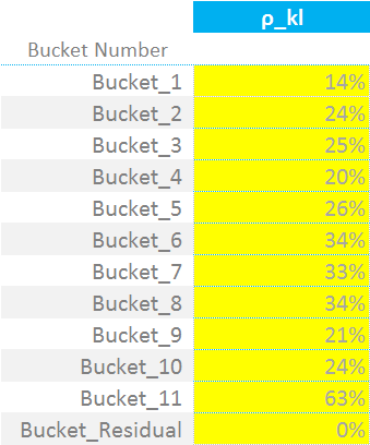
From an Excel perspective, we need to create a co-variance matrix that maps each security to all others. At first, we are interested in the within-bucket relationships, and all other co-variances are zero. The within-bucket correlations are calibrated by ISDA as per the below:
For each bucket, we must therefore calculate the appropriate co-variance between ISINs in the same bucket. This means deriving the co-variance matrices, according to which bucket each ISIN is in. As we see, for my example, I only have ISINs 5 and 13 in the same bucket – hence all of the zeros:
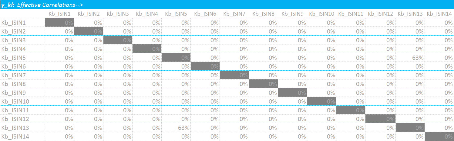
Showing;
- It is very easy to get confused between ISINs and Buckets here. I needed to make my input criteria as flexible as possible, therefore I wanted to allow for any ISIN being in any bucket. Less user-friendly implementations could just ask users to pre-define which bucket their securities are in.
- Sticking with my choice of implementation, it means I must define an array of the same size as my weighted sensitivities (WS’s, which is 1×14) for each ISIN.
- This array then defines the correlation between ISINs (or covariance…I use the terms interchangeably, be that right or wrong).
- Therefore, I can perform a simple sumproduct of the WS’s and the covariance matrix per ISIN.
This is how I implement the key formula that we keep on revisiting in these blogs:
\( \tag {2} K = \sqrt{\sum\limits_{k}{WS_{k}^2+{\sum\limits_{k}}{\sum\limits_{l≠k}{f_{kl}{ρ_{kl}}{WS_{k}}{WS_{l}}}}}}\)Where;
\( {WS_{k}}\) is the input sensitivity multiplied by the ISDA-supplied risk weighting.
\({f_{kl}}\) is the modification we have to make to our correlations in the case that one of the risk factors is above the Concentration Threshold. See my blog on this for more. For now, we assume we are below the CTs.
\({ρ_{kl}}\) is the correlation matrix that we just defined. It defines the correlation of the “WS” terms from one ISIN to the next (i.e. between k and l in the nomenclature). So for example, ISDA deem that ISINs falling within Bucket 11 have a correlation of 63% with each other. These are not currency dependent – one table serves all currencies.
I therefore calculate the value of “K” for each bucket, squaring the WS terms and adding in the sumproduct of correlation x WS:

Aggregating Positions across Risk Buckets
Now another small subtlety of the docs. The aggregation formula across buckets (equation 4 below) looks, at first pass, almost identical to the one for combining within a bucket (equation 2 above). But it is important to note that we must first calculate Sb for each bucket – as well as Kb above. We’ve defined Sb before:
\( \tag {3}{S_{b} = max(min({\sum\limits_{k}}WS_{k},K_{b}),-K_{b})}\)\( {S_{b}}\) is either the sum of all of the “Weighted Sensitivities” or the value of K for bucket b. We first take the smaller of the sum of the WS’s and then the larger of this and “negative K” for bucket b. This means that \( {S_{b}}\) can, in some instances, be a negative number.
Note that we do not calculate an Sb value for the Residual bucket (bucket 12 on my grid above).
We must now combine these calculated Sb values with the ISDA-supplied intra-bucket covariance matrix below:
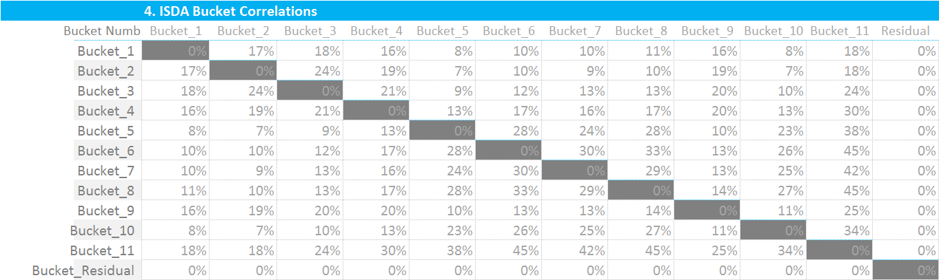
This final step is therefore nice and simple. We simply square each Kb value and add in the sumproduct of the Sb terms with their appropriate Bucket number in the covariance matrix. Put in equation-form:
\( {\tag {4} DeltaMargin = \sqrt{\sum\limits_{b}{K_{b}^2+{\sum\limits_{b}}{\sum\limits_{c≠b}{γ_{bc}}{S_{b}}{S_{c}}}}}+K_{residual}}\)Where;
\(γ_{bc}\) represents the “ISDA Bucket Correlations” matrix immediately above.
The full suite of calculations is below:
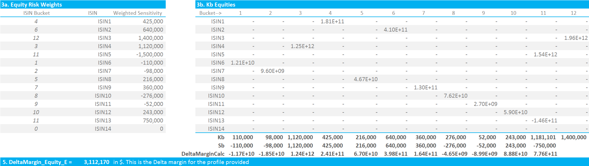
Et Voila! An ISDA SIMM Initial Margin amount of $3,112,170 for our relatively diverse array of securities.
In Summary
- We replicate the ISDA SIMM methodology in Excel for Equity Derivatives.
- The implementation is a little different to Rates, but overall is probably easier to achieve in Excel than for some other asset classes.
- We have looked at only 13 securities in our stylised example. We are sure that real portfolios will have many more, adding to the complexity from an Excel perspective.
- Still, it is clear that the SIMM model stays true to its’ guiding principles of speed, transparency and ease of replication. Even when your author is no expert for the asset class at hand!
- Remember to subscribe below for upcoming blogs covering Vega and Curvature margin for Equity Options.
- UPDATE: We now offer free 14-day trials for our SIMM for Excel product.