- We build an IM calculator in Excel for Swaptions under ISDA SIMM™.
- The methodology builds on the margin methodology for linear products, and uses very similar formulae.
- There are some subtleties around multiple currency portfolios that we expand upon.
- We also introduce the concept of Curvature Margin which is calculated via theta and lambda multipliers.
- UPDATE: We now offer free 14-day trials for our SIMM for Excel product
Swaptions Initial Margin
In my articles on ISDA SIMM™, I have looked at calculating Initial Margin for Uncleared Swaps for a few simple cases – USD Rates, Multiple Currency Portfolios and then I compare these to CCP margins.
Our goal with these blogs is to show that it can be a simple exercise to replicate the ISDA SIMM margin framework. So far, we have even performed all of the calculations in a simple Excel spreadsheet.
To date, I have only looked at linear products. Can I replicate the methodology under ISDA SIMM for Swaptions in an Excel spreadsheet? Read on to find out.
(Apologies to those who haven’t followed the previous ISDA SIMM in Excel blog, but to prevent myself repeating myself, I am going to take that blog as assumed prior reading for this blog).
1. Risk Sensitivities
The input for ISDA SIMM at each maturity is volatility multiplied by vega. We need to know what type of vol and the units of measurement, so we should be a little bit more explicit here:
\( \tag {1} VR = \sum σ \frac{dV}{dσ}\)Where;
VR = The Vega Risk input required for ISDA SIMM at each maturity point (tenor).
σ = The volatility at each tenor. The tenors are the same as used for Swaps. This volatility can be quoted as normal, log-normal or similar.
\(\frac {dV}{dσ}\) = change in price with a change in vol, commonly referred to as “vega”. We had a few fun and games with this in terms of defining the exact units it should be in. It is important to note that this is unscaled (at least for Interest Rates).
We now have a Microservice that generates these inputs for ISDA SIMM in a very simple manner in your web browser:
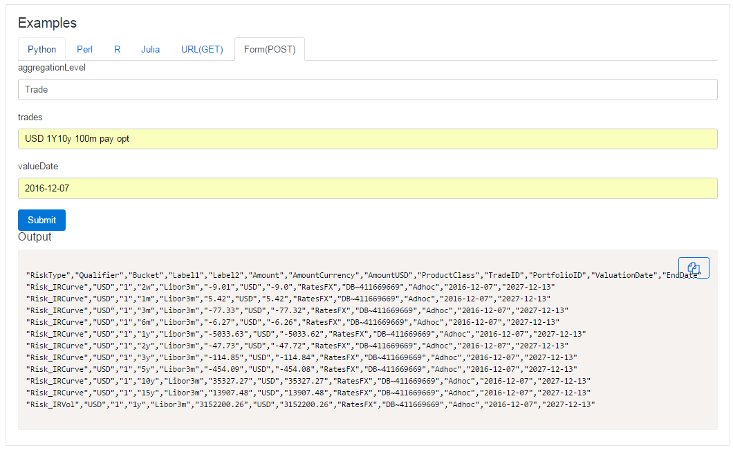
Showing;
- Our new page for calling a microservice that we use for testing. No scripting required – simply define your instrument (via free text, bloomberg tickers, Clarus short codes etc) and copy the output. In the absence of a Strike in the trade description, we will revert to the current break-even rate for the underlying swap.
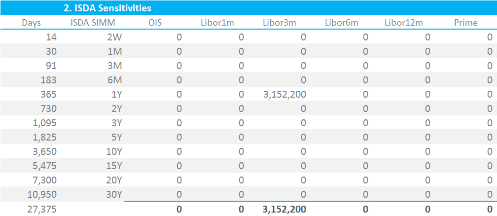
- For a 1y10y ATM USD Swaption in $100m notional, this gives us a Vega Risk of $3,152,200 to carry forward into our calculations and our spreadsheet – as shown below:
2. Risk Weightings
Sticking with the format of my original ISDA SIMM in Excel blog, we now apply Risk Weightings to every tenor that has a Vega Risk. To do this, ISDA makes reference to the Vega Concentration Risk, VCR. Please note that at the time of writing this blog, the Concentration Thresholds have not yet been defined. We therefore only have to multiply each Vega Risk by the Vega Risk Weight for Interest Rates:

I am using my underlying Swaps model to calculate ISDA SIMM for Swaptions. I therefore have retained multiple indices in my set-up per currency. Realistically, these are redundant – we will only have one column per currency.

3. Correlations
We now need to combine these per-tenor Vega Risk amounts into a margin number. This is more straight-forward than for swaps as we do not have to combine across sub-indices. The formula is virtually identical to last time:
\( \tag {2} K_{b} = \sqrt{\sum\limits_{k}{VR_{k}^2+{\sum\limits_{k}}{\sum\limits_{(l)≠(k)}{f_{kl}{ρ_{kl}}{VR_{k}}{VR_{l}}}}}}\)A couple of key notes on this formula:
- The Sum limits in this equation are over VR, the Vega Risk, instead of WS, the Weighted Sensitivity for Swaps. The equation is nonetheless fundamentally similar to the one for swaps.
- \( f_{kl} \) is defined as 1 for the Interest Rate risk class. To my mind, this is why the formula drops any reference to “i” – which for Swaps was the delta risk to different indices such as Libor3m, Libor6m, OIS etc. This means that we only have one “index” (a single vol surface for USD for example) and because \( f_{kl} \) is 1 we no longer need the “SubIndex” correlation matrix that I referred to in my previous blog.
- \( ρ_{kl} \) is the same correlation matrix as we used for Swaps:
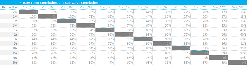
The use of the same correlation matrix was another motivating factor for keeping the structure of my spreadsheet for both Swaps and Swaptions very similar.
4. Calculate Vega IM
For a single currency Vega IM calculation, in Excel terms, we therefore implement the above equation by:
- Squaring all of the VR terms.
- Calculating the VR-weighted sumproduct at a single risk vertex for all VR‘s with the correlation matrix.
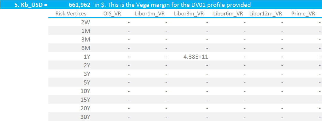
- Add together both of these terms and then take the square root. For a single currency portfolio, this is the Vega IM under ISDA SIMM.
ISDA refer to this as \( K_{b} \), which is the Vega IM for a single currency. Why isn’t it \( K_{v} \)? They ARE next to each other on a standard QWERTY keyboard, but….? Is this a standard short-hand I am not familiar with?
5. Multi-Currency Vega Margin
I stumbled a little bit at this point. In a similar manner to the FRTB documentation, the methodology now inexplicably (to me) drops all reference to currencies. For swaps, the document is very clear how to combine Delta Margin across different currencies. For Vega Margin, I found it less clear. We are instead left to interpret a “bucket” as a currency:
\( \tag {3} Vega Margin = \sqrt{\sum\limits_{b}{K_{b}^2+{\sum\limits_{b}}{\sum\limits_{(c)≠(b)}{γ_{bc}{g_{bc}}{S_{b}}{S_{c}}}}}}\)Where;
\( {S_{b}}\) is either the sum of all of the “VR” terms or the value of \( K_{b} \) for currency b. We first take the smaller of the sum of the VR‘s and then the larger of this and “\( K_{b} \)” for currency b. This means that \( {S_{b}}\) can, in some instances, be a negative number.
\( {γ_{bc}}\) is calibrated by ISDA. It is set at 27% according to the documentation here.
\( {g_{bc}}\) is calibrated according to Concentration Risk in each currency. As at the time of writing, this is yet to be implemented by ISDA.
As I said in a previous blog, a portfolio may therefore have a total Vega Margin that is lower than a simple sum across all currencies of the individual \( K_{b} \) values, highlighting the offsetting nature of some of the risks.
6. Curvature Risk
And now for something completely new. Apologies this comes after 1,000 words, but it’s best to have a single page of reference for all things Swaptions.
We must now add Curvature Margin to this Vega Margin number, to arrive at the overall Margin number for a Swaption. This seems to allow for the fact that gamma (change in delta with a change in price) is not provided for anywhere else in the model.
The core equations are again very similar to dealing with the WS terms for swaps and the VR terms for swaptions. First, we calculate the Curvature Risk:
\( \tag {4} CVR_{ik} = \sum\limits_{j} SF(t_{kj}) σ_{kj} \frac{dV_{i}}{dσ}\)Where;
\( SF(t_{kj}) \) is a new term for us. In our first screenshot today, we said it was important to include the number of days for each tenor point. This is so that we can calculate the value of SF. At each tenor, SF is simply equal to:
SF = 0.5 * minimum(1, 14/(maturity in days))
ISDA provide the values of SF, so it is pretty straightforward to end up with another matrix of values, this time CVRs:

The grid is pretty simple – just multiplying the Vega Risk from step 1 by the SF in the right-hand column.
7. Curvature Risk Weightings
To calculate the Curvature Risk Weightings, we need to take the correlation matrix, \( ρ_{kl} \), and square the values:
\( \tag {5} K_{b} = \sqrt{\sum\limits_{k}{CVR_{b,k}^2+{\sum\limits_{k}}{\sum\limits_{(l)≠(k)}{{ρ_{kl}^2}{CVR_{b,k}}{CVR_{b,l}}}}}}\)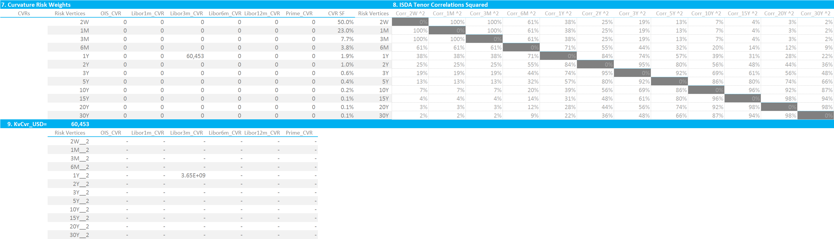
8. Calculate Curvature IM
Again, we fall back on a familiar equation. To calculate the total Curvature IM we use broadly the same formula as we use to calculate multi-currency IM. The difference being the introduction of a new term, λ, and again using a square term on our correlation co-efficient:
\( \tag {6} Curvature Margin = \sum\limits_{b,k}{CVR_{b,k}+λ\sqrt{\sum\limits_{b}{K_{b}^2+{\sum\limits_{b}}{\sum\limits_{(c)≠(b)}{γ_{bc}^2}{S_{b}}{S_{c}}}}}}\)with the above term floored at zero.
I won’t dwell too much on this final equation – if you have got this far, you can almost certainly work through this final step!
However, the documentation is vague as to how to calculate λ for multi currency portfolios, so I will try to help out here.
\( λ = (2.58^2 -1)(1+θ) – θ, \)
where;
\( \tag {7} θ = \frac{\sum\limits_{b,k}CVR_{b,k}}{\sum\limits_{b,k}|CVR_{b,k}|}\)Equation (7) is this time capped at zero.
Both θ and λ are trivial to calculate once you are familiar with the terminology. Here are a couple of pointers:
- The “2.58” is a placeholder for the Excel formula “NORMSINV(0.995)”. This is the 99.5th percentile of the standard normal distribution.
- You must calculate θ and λ on a global basis for multi-currency portfolios. This means summing all of the Curvature Risk Weight values across all currencies, as well as summing their absolute values.
- The value of θ for our $100m 1y10y ATM Swaption is zero.
- The value of λ is 5.6348966.
9. One final “gotcha”
Finally, the result from Equation (6) must be multiplied by 2.3 for Interest Rate products. This gives us a final Curvature Margin for a $100m 1y10y ATM Swaption of $922,531.
Adding together with the Vega Margin of $661,962, means that the margin (excluding the delta) for the Swaption is $1,584,493.
Finally…
As a sanity check for this value, CME kindly provided us with a few IM examples for their cleared product.
Remember that to perform a fair comparison, we must include the delta of the swaption. Because this swaption is ATM, our delta is ~$43,500, with a fair amount of bleed across the buckets due to the forward start nature. This gives us an ISDA SIMM IM for the delta alone of $2.02m. Adding in the option-related components gives us a total IM requirement of $3.60m.
The CME margin is just over half of this, with even more substantial savings if the delta hedge is also cleared there.
We will look further into these comparisons in future blogs.