Principal Component Analysis (PCA) is a well-known statistical technique from multivariate analysis used in managing and explaining interest rate risk. Before applying the technique it can be useful to first inspect the swap curve over a period time and make qualitative observations.
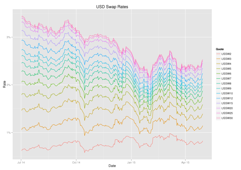
By inspection of the swap curve paths above we can see that;
1. Prices of swaps are generally moving together,
2. Longer dated swap prices are moving in almost complete unison,
3. Shorter dated swap price movements are slightly subdued compared to longer dated swap prices,
4. Paths are not crossing, so the curve is upward sloping in our period of observation.
The following box-and-whiskers view of the same data gives a flavour of both rate level and dispersion during the period of observation.
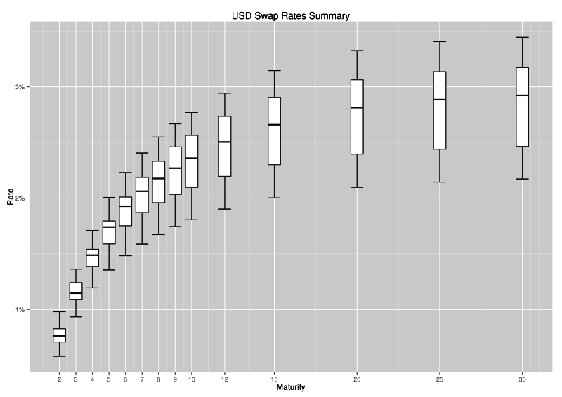
(In a box and whiskers plot, the centre line in the box is the median, the edges of the box are the lower and upper quartiles (25th and 75th percentile), whilst the whiskers highlight the last data point within a distance of 1.5 x (upper – lower quartile) from the lower and upper quartiles. Values outside the whiskers are plotted separately as dots and suspected to be outliers.)
Analysis of Rate Changes
From a risk management perspective it is interesting to look not only at levels, but also at (daily) returns. Since interest rates are low, we consider absolute returns.
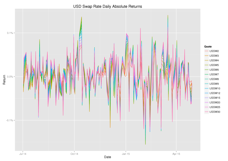
It is clear from the graph that absolute returns are highly correlated across the maturities and fairly stationary, suggesting the data is ripe for principal component analysis.
Finally, another view that I find interesting is the change in prices of local butterfly (1:2:1) swap packages.
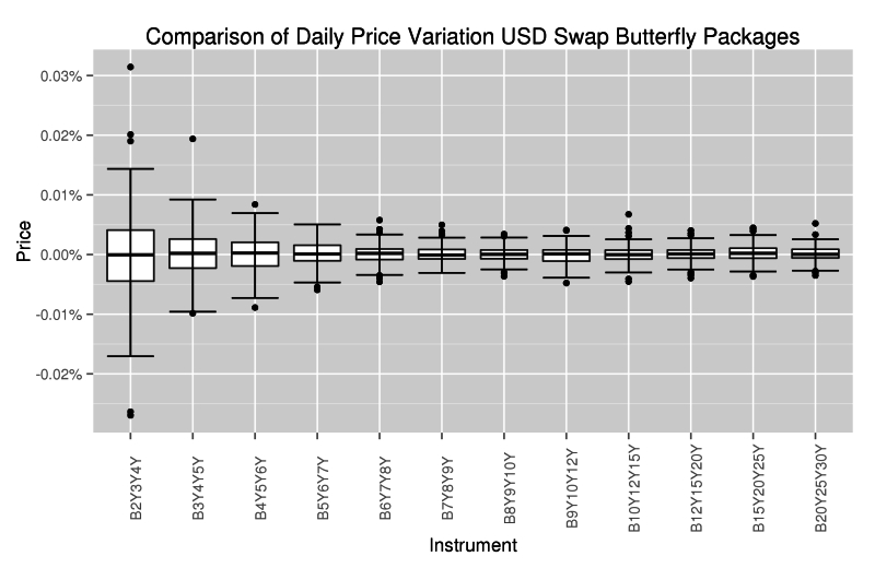
The graph shows that much more flexing of the curve occurs at the shorter end (2Y-5Y), the region that overlaps with the Eurodollar futures market.
PCA Decomposition
The central idea of principal component analysis (PCA) is to reduce the dimensionality of a data set consisting of a large number of interrelated variables, while retaining as much as possible of the variation present in the data set. This is achieved by transforming to a new set of variables, the principal components (PCs), which are uncorrelated, and which are ordered so that the first few retain most of the variation present in all of the original variables.
Applying PCA in our context reveals an expression for the daily returns of the form;
$$
\begin{eqnarray}
\text{USSW2}(T-1,T) &=& \alpha_{2} X_1 &+& \beta_2 X_2 &+& \gamma_{2} X_3 + …\\
\text{USSW3}(T-1,T) &=& \alpha_{3} X_1 &+& \beta_3 X_2 &+& \gamma_{3} X_3 + …\\
\vdots &=& \vdots \\
\text{USSW30}(T-1,T) &=& \alpha_{30} X_1 &+& \beta_{30} X_2 &+& \gamma_{30} X_3 + …
\end{eqnarray}
$$
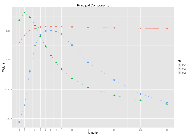
where, \(\text{USSWn}(T-1,T)\) denotes the daily return on the nY swap price. The variables \(X_1, X_2\) and \(X_3\) are the new uncorrelated (random) variables, the principal components, whilst the constants \(\alpha_{i}, \beta_{i}\) and \(\gamma_{i}\) are the so-called principal component ‘loadings’ or ‘weights’ or ‘coefficients’. A confusion can arise in terminology at this point, the loadings associated with each principal component are of such interest that it is not uncommon to refer to the loadings as the principal components. As an example the second graph below shows the principal component loadings and we used a title of simply ‘Principal Components’ and labelled the loadings PC1, PC2, and PC3 when a title of ‘Principal Component Loadings’ and labels PCL1, PCL2 and PCL3 would be more precise.
On our example data PCA yields the following decomposition;
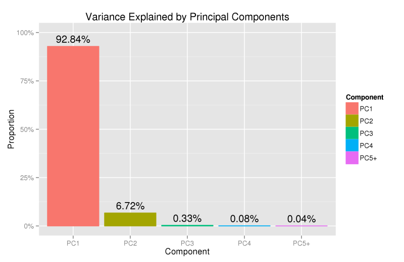
The PCA results above show that over 92% of the variance in daily changes of swap prices is explained by a single component, a near parallel movement in rates and quantifies our initial qualitative observation that the longer rates are moving in almost complete unison, whilst the shorter end is slightly subdued. Most of the remaining variance is explained by the second component, a ‘seesaw-like’ rotation around the 9Y point. Together, the first three components explain 99.9% of the total variance and are commonly identified and referred to as level, slope and curvature.
To appreciate the terms, level, slope and curvature, it can be useful to look at changes in sign of the principal component loadings in the graph above. PC1 has the same sign for each maturity, so all rates will move up or down together due to the first principal component (level). PC2 has one change in sign, so the shorter maturity rates will move in opposite direction to the longer rates due to the second principal component (slope). PC3 has two changes in sign, so the shortest and longest maturities move in the same direction, whilst the middle maturities move in the opposite direction (curvature).
Swap Rates or Forward Rates?
In the example above we analysed swap rates, it is no surprise they are highly correlated across maturity, since each swap completely contains each shorter maturity swap. It is quite natural to ask if a similar compression to 3 factors would be revealed if we analysed the movements of non-overlapping forward rates. Lekkos (2000) considered this idea and found that many more factors are needed and there was no natural interpretation of level, slope and curvature. However, Lord and Pelsser (2007) looked at the same problem and found that PCA of forward rates is quite sensitive to interpolation methods used to construct them, and suggested that the mostly likely explanation for Lekkos’ result was a poor choice of interpolation. Lord and Pelsser showed that, with careful choice in interpolation method, one could indeed explain forward rate movements in 3 factors which had a natural interpretation of level, slope and curvature.
Level, Slope, Curvature: Fact or Artefact?
As level, slope and curvature movements are commonly identified in the analysis of interest rate curves, one might wonder if that is always the case or what conditions are required to cause such a decomposition. The paper of Lord and Pelsser (2007) investigated this idea and established some positive results for sufficiency, concluding that
“… the level, slope and curvature pattern is part fact, and part artefact. It is caused both by order and positive correlations present in terms structures (fact), as well as by the orthogonality of the factors and the smooth input we use to estimate correlation (artefact).”
Practical Applications
Principal component analysis can used in the following areas;
1. PnL Explain – rates pnl can be explained as level, slope, curvature and residual,
2. Hedging – portfolio hedging can be determined by neutralising the movements in the first few principal components,
3. Relative Value Analysis – richness/cheapness of the curve can be monitored by PCA residuals,
4. Scenario Analysis – principal components can help construct realistic scenarios for risk management purposes.
Bibliography
- Credit Suisse (2012), “PCA Unleashed”.
- Jolliffe, I.T. (2002), “Principal Component Analysis”.
- Lardic, S. et al. (2003), “PCA of the yield curve dynamics: questions of methodologies”, Journal of Bond Trading and Management, 1.
- Lekkos, I. (2000), “A critique of factor analysis of interest rates”, Journal of Derivatives, 8(1).
- Lord, R. and Pelsser, A. (2007), “Level-Slope-Curvature–Fact or Artefact?”, Applied Mathematical Finance, 14 (2).
- Salomon Smith Barney, (2000), “Principles of Principal Components: A fresh look at Risk, Hedging, and Relative Value”.
- Standard Chartered (2013), “Introducing a relative value tool for swaps”.
- TD Securities (2015), “Market Musings — Relative Value Across the U.S. Swap Surface: A PCA Approach”.
Update 22nd August 2017: Added reference to the TD Securities report.