 The SABR model is widely used, particularly in the interest rate world, to help manage the volatility smile. Depending on 4 parameters, \(\alpha\), \(\beta\), \(\rho\) and \(\nu\), often \(\beta\) is considered a fixed constant whilst the other 3 parameters are calibrated to liquid market prices. There tends to be two types of calibration algorithms; local such as Levenberg-Marquardt, and global such as differential evolution. Local calibration approaches tend to work well if one has a good initial guess, however it is not that obvious how to get a good initial guess. A practical approach is to assume yesterday’s smile parameters, \(\nu\) and \(\rho\) (or some average of recent parameters), and then determine \(\alpha\) from the latest ATM quote. The idea being that whilst the level (\(\alpha\)) may change day to day, one hopes that the smile parameters are relatively stable.
An alternative, requiring no more than high-school algebra, is to look at the taylor expansion of the infamous SABR formula. As Hagan et. al. noted in their original paper,
“The complexity of the above formula for \(\sigma_B(K,f)\) obscures the qualitative behavior of the SABR model. To make the model’s phenomenology and dynamics more transparent, note that formula (2.17a – 2.17c) can be approximated as
$$\sigma_B(K,f)=\frac{\alpha}{f^{1-\beta}}\left\{1-\frac{1}{2}(1-\beta-\rho\lambda)\log K/f + \frac{1}{12}\left[(1-\beta)^2+(2-3\rho^2)\lambda^2\right]\log^2 K/f + …\right. $$
provided the strike \(K\) is not too far away from the current forward \(f\). [Note that \(\lambda=\frac{\nu}{\alpha}f^{1-\beta}\)]
The complexity of the SABR formula also makes it tricky to make a good initial guess, although the paper of Gauthier and Rivaille, “Fitting the Smile, Smart Parameters for SABR and Heston”, makes a very good effort. However, the simplicity of the taylor expansion reveals a simple and explicit initial guess that happens to be good enough for local calibration routines and is described next.
Suppose that one can extract a reasonable description of the curvature of the smile near the current forward, \(f\), from the market quotes; that is, suppose we can extract a function,
$$\sigma_B(K,f)= a + b z + c z^2$$
where, \(z=\log K/f\). The extraction of this function requires some care, and different approaches can be taken depending on the quality of the data. Then one simply matches terms,
$$ a = \frac{\alpha}{f^{1-\beta}}$$
$$ b = -\frac{\alpha}{f^{1-\beta}}\frac{1}{2}(1-\beta-\rho\lambda) $$
$$ c = \frac{\alpha}{f^{1-\beta}}\frac{1}{12}\left[(1-\beta)^2+(2-3\rho^2)\lambda^2\right]$$
Now since \(\beta\) is already known, \(\alpha\) is revealed immediately, and we are left with two equations and two unknowns. Working through the high-school algebra, reveals \(\rho\) and \(\nu\) explicitly, and thus an initial guess matching the market quotes near the current forward \(f\)!!
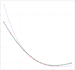
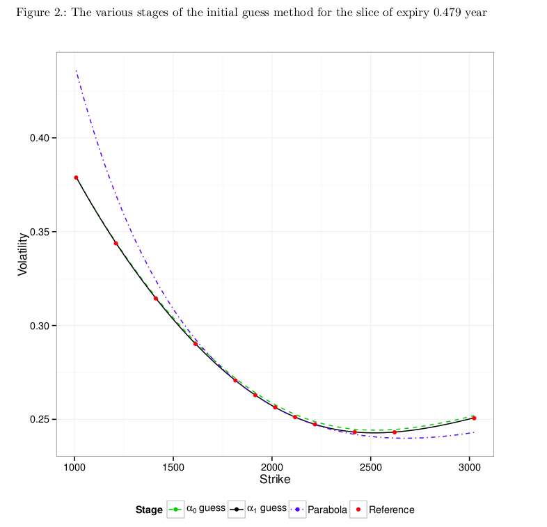
An example of the process is shown below, the blue dashed line is the parabola approximating the market quotes near the forward, and the green dashed line is the SABR model based only on this initial guess. As one can see the initial guess is remarkably close to the market quotes (red dots).
So far we have only considered the lognormal version of Hagan formula, a similar approach will work if one looks at the taylor expansion of the normal volatility version of Hagan formula, which may be more convenient when working with BpVol based market quotes. The details have been written up in this note with Fabien Le Floc’h, Explicit SABR Calibration Through Simple Expansions
.
Update 19-Aug-2014
I have noticed the same basic idea is present in Effective Forward Volatility by Andreason and Huge in the context of their extension of the classic SABR model (Eqn. 36 and 37), although not present in the earlier version of the paper, ZABR–Expansions for the masses.