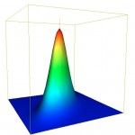
 Using Java I implemented the double precision algorithm to compute the cumulative trivariate normal distribution found in A.Genz, Numerical computation of rectangular bivariate and trivariate normal and t probabilities”, Statistics and Computing, 14, (3), 2004. The cumulative trivariate normal is needed to price window barrier options, see G.F. Armstrong, Valuation formulae for window barrier options”, Applied Mathematical Finance, 8, 2001.
$$\Phi({\bf b},{\bf R}) = \frac{1}{(2\pi)^{3/2}|{\bf R}|^{1/2}} \int_{-\infty}^{b_1}\int_{-\infty}^{b_2}\int_{-\infty}^{b_3} \exp\left(\frac{-{\bf x}^T {\bf R}^{-1} {\bf x}}{2}\right)dx_3 dx_2 dx_1,$$
where \(b = (b_1, b_2, b_3)\) and \( {\bf R} = (\rho_{ij})\) is the correlation matrix.
It was hard to validate my implementation because I could not find analytical results or a set of reference results. Even the famous collection of mathematical tables in Abromowitz and Stegun: Handbook of Mathematical Functions did not have a set of values. So, I implemented unit tests to cover all branches of the code and compared these results with results from an R script that uses the mvnorm library (Monte Carlo, 1,000,000,000 trials). Below is a minimal set of test cases with complete code coverage, assuming we already have the univariate and bivariate norms validated, see the earlier post Test data for the cumulative bivariate normal distribution.
| \(b_1\) | \(b_2\) | \(b_3\) | \(\rho_{12}\) | \(\rho_{13}\) | \(\rho_{23}\) | Code Branch | Java | R | |
|---|---|---|---|---|---|---|---|---|---|
| 1 | 0 | 0 | 0 | 0 | 0 | 0 | \(|b_1|+|b_2|+|b_3|\lt\epsilon\) | 0.125 | 0.125 |
| 2 | -0.5 | 0.4 | 0.5 | 0 | 0 | 0 | \(|\rho_{12}|+|\rho_{13}|\lt\epsilon\) | 0.13982906773123424 | 0.139829067731234 |
| 3 | -0.5 | 0.4 | 0.5 | 0.001 | 0.001 | 1.0 | \(1-\rho_{23}\lt\epsilon\) | 0.2023518531793232 | 0.202351853167879 |
| 4 | -0.5 | 0.4 | 0.5 | -0.1 | 0.1 | -1.0 | \(\rho_{23}+1\lt\epsilon , b_2\gt-b_3\) | 0.10616785383590192 | 0.10616785392407 |
| 5 | -0.5 | -0.4 | 0.5 | -0.1 | 0.1 | -1.0 | \(\rho_{23}+1\lt\epsilon , b_2\leq-b_3\) | 0.0 | 0.0 |
| 6 | 1 | 7 | 8 | 0.0001 | 0.8 | 0.6 | Edge case | 0.8413447460674663 | 0.841344746067466 |
| 7 | 0.1 | 1.4 | 1 | 0.1 | 0 | 0.5 | Typical case | 0.43470997627360936 | 0.434709976275275 |
| 8 | 1 | 0.1 | 1.4 | 0.5 | 0.1 | 0 | Typical case | 0.4640394315336022 | 0.464039431577782 |
#R script to generate cumulative trivariate norm test values
library(mvtnorm)

options(digits=15)
ntrials = 1000000000
error   = 0.0000000001

lower <- c(-Inf,-Inf,-Inf)
upper <- c(0,0,0)
corr = matrix( c(1,0,0,0,1,0,0,0,1), nrow = 3, ncol = 3)

#Special Cases
#1. |H1| + |H2| + |H3| < MachineEpsilon
upper <- c(0,0,0)
corr = matrix( c(1,0,0,0,1,0,0,0,1), nrow = 3, ncol = 3)
prop1 <- pmvnorm(lower,upper,mean, corr,NULL,GenzBretz(ntrials,error,0))

#2. |R12| + |R13| < MachineEpsilon
upper <- c(-0.5,0.4,0.5)
prop2 <- pmvnorm(lower,upper,mean, corr,NULL,GenzBretz(ntrials,error,0))

#3. 1-R23 < MachineEpsilon
corr[1,2]<- 0.001 -> corr[2,1]
corr[1,3]<- 0.001 -> corr[3,1]
corr[2,3]<- 1.0 -> corr[3,2]
corr
prop3 <- pmvnorm(lower,upper,mean, corr,NULL,GenzBretz(ntrials,error,0))

#4. R23+1 < MachineEpsilon
corr[1,2] <- -0.1 -> corr[2,1]
corr[1,3] <- 0.1  -> corr[3,1]
corr[2,3] <- -1.0 -> corr[3,2]
prop4 <- pmvnorm(lower,upper,mean, corr,NULL,GenzBretz(ntrials,error,0))

#5. H2<=-H3
upper[3] <- -0.4
prop5 <- pmvnorm(lower,upper,mean, corr,NULL,GenzBretz(ntrials,error,0))

#6. Edge cases
corr[1,2] <- 0.0001 -> corr[2,1]
corr[1,3] <- 0.8 -> corr[3,1]
corr[2,3] <- 0.6 -> corr[3,2]
prop6 <- pmvnorm(lower,upper,mean, corr,NULL,GenzBretz(ntrials,error,0))

# Normal Cases
# 7. normal case
upper = c(0.1,1.4,1)
corr[1,2] <- 0.1 -> corr[2,1]
corr[1,3] <- 0 -> corr[3,1]
corr[2,3] <- 0.5 -> corr[3,2]
prop7 <- pmvnorm(lower,upper,mean, corr,NULL,GenzBretz(ntrials,error,0))

#8. normal case
upper = c(1,0.1,1.4)
corr[1,2] <- 0.5 -> corr[2,1]
corr[1,3] <- 0.1 -> corr[3,1]
corr[2,3] <- 0 -> corr[3,2]
prop8 <- pmvnorm(lower,upper,mean, corr,NULL,GenzBretz(ntrials,error,0))

#Print Results
prop1
prop2
prop3
prop4
prop5
prop6
prop7
prop8
This article was authored by Liam Henry.
