FRTB – Basic Approach for CVA

Introduction

A core component of managing bilateral exposures is CVA – Credit Valuation Adjustment.

The grandfather of all XVAs, it describes the change in exposure we have to a counterparty as a result of changes in both the mark-to-market of a derivative and the change in credit-worthiness of our counterparty.

Today, we’ll look at the capital required to be held against CVA risk.

Basel d424

Basel III: Finalising Post-Crisis Reforms was last updated on 7th December 2017. We are interested today in the third section “Minimum capital requirements for CVA risk”. It’s worth dwelling a little bit on why;

• According to the BCBS, Credit Valuation Adjustment reflects the “adjustment of default risk-free prices of derivatives due to a potential default of the counterparty”. It excludes “DVA” i.e. the effect of the bank’s own default.
• CVA risk is “the risk of losses arising from changes in counterparty credit spreads and market risk factors that drive prices of transactions”.
• Trades with a CCP (strictly, a QCCP) are exempt from CVA capital requirements.
• The FRTB covers how much capital must be held versus the “CVA portfolio”. This is all other derivatives held, plus any “eligible CVA hedges”. (Are these CVA hedges therefore not necessarily derivatives?).
• There are two approaches to measuring CVA – the Basic Approach (BA-CVA) and, subject to regulatory approval, the Standardised Approach (SA-CVA).

We will only look at the Basic Approach today as, despite the name, it is pretty involved!

Basic Approach to CVA

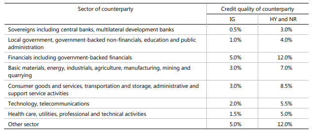
The Standalone CVA Capital is designated as SCVA. It is governed by the Risk Weight for the counterparty – this risk should, in theory, reflect the volatility of its’ credit spread. These risk weights are shown below:

Showing;

• Risk Weights (RW) are defined by credit quality and sector.
• A counterparty is classified as either investment grade (IG), high yield (HY) or not rated (NR).

Armed with these Risk Weights, we can introduce our first (and most important) equation – how to calculate the individual CVA capital required for a given counterparty, C.

The capital CVA charge is calculated across all netting sets (NS) versus the counterparty (C), and is based on the effective maturity (M) multiplied by the exposure at default (EAD), adjusted by a supervisory discount factor (DF).

Mathematically;

\( \tag {1} SCVA_{c} = \frac{1}{α}.RW_{c}.\sum\limits_{NS}{M_{NS}}.EAD_{NS}.DF_{NS}\)

Where;

α = 1.4

NS is a Netting Set. So we basically sum up all of these calculations across all of the netting sets for a given counterparty.

M is the “effective maturity for the netting set”. We’ve got to refer to Basel II to calculate this – please see section below.

EAD is the Exposure at Default – calculated using either CEM (soon to be SA-CCR) or via your own Internal Model. Using an Internal Model really complicates matters (see for example the calculations below for M!).

RW for Counterparty C is the Risk Weight according to the table above – i.e. ranging from 0.5% for Central Banks and Sovereigns, up to 12% for un-rated counterparties.

DF is a supervisory discount factor – which is equal to 1 if you are on Internal Models. Otherwise, you need to use the natural log of M:

\( \tag {2} DF_{NS} = \frac{1-e^{-0.05.M_{NS}}}{0.05.M_{NS}}\)

Read on to find more about this M term (the “effective maturity of the netting set”) and why it’s really the pivotal point of the calculations.

M, Effective Maturity of a Portfolio

First things first – if you are not using Internal Models for Credit (i.e. you are using CEM or will be using SA-CCR) then this is really simple. Your Effective Maturity, M,  is equal to the weighted average maturity of the cashflows:

\( \tag {3} Effective Maturity, M = \frac{\sum\limits_{t}{t*CF_{t}}}{\sum\limits_{t}{CF_{t}}}\)

where CF are the contractually agreed to cash-flows and t is time until the cashflow.

However, if you are on Internal Models for Credit, you are somewhat on your own. According to “Paragraphs 38 and 39 of Annex 4 of Basel II” Effective Maturity, M, is equal to:

 

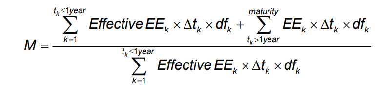
This isn’t straight-forward, so you can dig more into this on pages 261-263 of the original Basel II framework here. I will simply summarise the steps as I understand them.

1. Use your market data set (including vol surfaces) to project where the mark-to-markets of the counterparty portfolio could go for e.g. each day/month over the next year.
2. Use your probability distribution to then “average” the values across different possible future values of the market risk factors for each time, t. This is your “Effective EE” from above.
3. These “Effective EE” terms are then summed up according to their time from today (Δt), discounted by the risk free rate (df).
4. The EE terms are summed differently according to whether they mature under 1 year – where you only take values until they mature. Or if over one year, you take all of the values.
5. These are then divided by all of the EE‘s that are maturing within one year to give you an “Effective Maturity”.

The final Effective Maturity, M, can now be plugged back into equation (1) above to calculate the SCVA for a given counterparty.

Still with me at the back? Let’s hope most of our readers are on Internal Models so don’t have to bother with the above steps!

Consolidate the results across counterparties

We must now consolidate the standalone CVA capital charges across multiple counterparties. This involves the BCBS calibrating a “supervisory correlation parameter” to apply to CVAs across different counterparties.

The equation they choose to employ is:

\( \tag {4} K_{reduced} = \sqrt{(ρ.\sum\limits_{c}{SCVA_{c}})^2+(1-ρ^2).\sum\limits_{c}{SCVA_{c}}^2}\)

This gives you the capital requirement (K). It is based on the standalone capital requirement for each counterparty (SCVA) and is multiplied by ρ as per the equation above. The BCBS have calibrated ρ to 50%.

In Summary

• Calculating regulatory capital that is required to be held versus CVA risk can be done in a number of ways.
• We have started with the “Basic Approach” – BA-CVA.
• This is a 3 step process, whereby we must project potential exposures to a counterparty, multiply these by regulatory-defined Risk Weights, and then consolidate over multiple counterparties.
• The BCBS define the Risk Weights and the cross-counterparty correlations.
• The most involved piece of work is to project potential counterparty exposures, especially if you are on an Internal Model.
• We’ll take a look in the future at the Standardised Approach (SA-CVA) to see how it differs.