On 1 January 2017, the Standardised approach for measuring counterparty credit risk exposures (SA-CCR) will take effect. SA-CCR is required for Credit Risk Capital, as well as Exposures to CCPs and the Leverage Ratio. It is particularly important for Derivatives as it provides for improved netting benefit and recognition of margin for both cleared and bi-lateral trades.
In this article I will look at the SA-CCR methodology as applicable to interest rate swaps.
UPDATE: We now offer free 14-day trials for our SA-CCR for Excel product
Background
In March 2014, the Basel Committee on Banking Supervision (BCBS) published is Standardised Approach (SA-CCR) for measuring exposure at default (EAD) for counterparty credit risk (CCR). The full document is here. SA-CCR replaces the current non-internal model approaches, the Current Exposure Method (CEM) of 1995 and the Standardised Method (SM) of 2005. The majority of banks use CEM as relatively few firms have Internal Model Method (IMM) approval from their regulator.
Exposure at Default
Exposure at Default (EAD) is calculated for each counterparty using the formula:
![]()
where alpha equal 1.4, RC is Replacement Cost and PFE is Potential Future Exposure.
Replacement Cost captures the loss that would occur if a counterparty were to default and was closed out of it’s transactions immediately.
Potential Future Exposure add-on represents an potential increase in exposure over a 1-year time horizon for unmargined transactions or a MPOR of 5d, 10d or 20d for margined transactions.
Replacement Cost (RC)
Replacement Cost is calculated at the netting set level, so positive and negative mark-to-markets (MTMs) of trades are offset only when they are within the same netting set.
Recall that exposure is when the counterparty owes us (positive MTM) and not when we owe the counterparty (negative MTM) and we can only use the negative MTM trades to offset positive MTMs, when they are both under the same Netting Agreement and so subject to novation.
For unmargined transactions, the Replacement Cost formula is:
![]()
where V is the sum of the MTMs of derivative transactions in the netting set and,
C is the haircut value of net collateral held, where the haircut reflects the potential change in value of non-cash collateral over a 1-year time period. For non-cash collateral received from the counterparty the value is decreased using a haircut (e.g. 10%) while non-cash collateral posted to the counterparty is increased by the haircut.
For margined transactions, the formula is:
![]()
where V and C are as before, and the term TH + MTA – NICA represents the largest exposure that would not trigger a VM call and it contains levels of collateral that need to be always maintained.
TH is the positive threshold before the counterparty must send us collateral and MTA is the minimum transfer amount, both of which are zero for Clearing and are usually non-zero for ISDA CSAs.
NICA is Net Independent Collateral Amount and represents the the collateral (other than VM) posted by the counterparty that we may keep upon default, the amount of which does not change in response to the value of transactions it secures and/or the Independent Amount (IA) parameter as defined in ISDA documentation, less any unsegregated collateral posted by us to the counterparty.
Potential Future Exposure (PFE)
PFE add-ons are calculated for each asset class within a netting set and then aggregated. Add-ons for an asset class require the use of hedging sets, which are transactions within a single netting set within which partial or full offsetting is recognised in the methodology.
For Interest rate derivatives a hedging set consists of all derivatives that reference interest rates of the same currency such as USD, EUR, JPY, etc. Hedging sets are further divided into maturity categories. Long and short positions in the same hedging set are permitted to fully offset each other within maturity categories; across maturity categories, partial offset is recognised.
Interest Rate Basis Swaps must be in separate hedging sets for each pair of risk factors, so Libor 3m vs 6m form a single hedging set, one that is distinct from Libor 1m vs 3m and FedFunds vs Libor 3m.
The PFE add-on formula is:
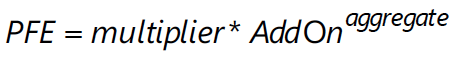
Multiplier
The multiplier in the PFE formula serves to reduce the add-on for over collateralisation as in practice many banks hold excess collateral precisely to offset potential increases in exposure represented by the add-on.
From the bcbs279 document:
148. For prudential reasons, the Basel Committee decided to apply a multiplier to the PFE component that decreases as excess collateral increases, without reaching zero (the multiplier is floored at 5% of the PFE add-on). When the collateral held is less than the net market value of the derivative contracts (“under-collateralisation”), the current replacement cost is positive and the multiplier is equal to one. Where the collateral held is greater than the net market value of the derivative contracts (“over-collateralisation”), the current replacement cost is zero and the multiplier is less than one (i.e. the PFE component is less than the full value of the aggregate add-on).
The formula for the multiplier is:
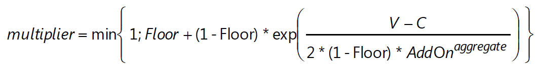
where Floor is 5%, V is the value of the derivative transactions in the netting set, and C is the haircut value of net collateral held.
Aggregate AddOn
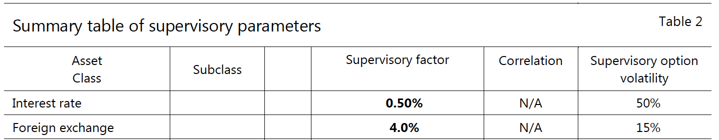
Diversification benefits across asset classes are not recognised. Instead, the respective add-ons for each asset class are simply aggregated. There are five asset classes; interest rate, foreign exchange, credit, equity or commodity and a derivatives transaction is assigned to an asset class based on its primary risk driver.
Most derivative transactions have one primary risk driver, defined by its reference underlying instrument (e.g. an interest rate curve for an interest rate swap or a reference entity for a credit default swap) and will fall into one asset class.
Complex or hybrid derivatives may be required to be allocated to more than one asset class.
AddOn Calculation Steps
In general the steps are as follows:
- An adjusted notional amount based on actual notional or price is calculated at the trade level.
- A maturity factor (MF) reflecting the time horizon appropriate for the type of transaction is calculated at the trade level and is applied to the adjusted notional.
- A supervisory delta adjustment is made to this trade-level adjusted notional amount based on the position (long or short) and whether the trade is an option, CDO tranche or neither, resulting in an effective notional amount.
- A supervisory factor (SF) is applied to each effective notional amount to reflect volatility.
- The trades within each asset class are separated into hedging sets and an aggregation method is applied to aggregate all the trade-level inputs at the hedging set level and finally at the asset-class level. For credit, equity and commodity derivatives, this involves the application of a supervisory correlation parameter to capture important basis risks and diversification.
Adjusted Notional
For interest rate and credit derivatives, the trade-level adjusted notional is the product of the trade notional amount, converted to the domestic currency, and the supervisory duration (SD) which is given by the following formula:
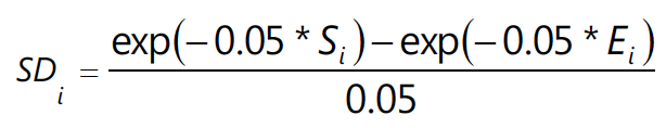
where S is the time period in years from today to the start date of the derivative (zero if in the past) and E is the time period in years from today to the end date of the derivative trade.
For variable notional swaps such as amortising and accreting swaps, banks must use the average notional over the remaining life of the swap as the trade notional amount.
Maturity Factor (MF)
For unmargined transactions, the MF is the lesser of one year and remaining maturity of the derivative contract, floored at ten business days.
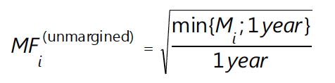
where Mi is the transaction i remaining maturity (in years) floored by 10 business days.
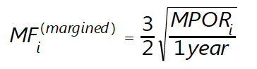
For margined transactions, the MPOR is:
- Five business days for centrally cleared derivative transactions subject to daily margin agreements.
- At least ten business days for non-centrally-cleared derivative transactions subject to daily margin agreements.
- Twenty business days for netting sets consisting of 5,000 transactions that are not with a CCP.
- Double the MPOR for netting sets with outstanding disputes
And then MF is given by:
Supervisory delta adjustments
These parameters are also defined at the trade level and are applied to the adjusted notional amounts to reflect the direction of the transaction and its non-linearity. For derivatives that are not options or CDO tranches, the value of this parameter is +1 for long (MTM increases when the value of the primary risk factor increases) or -1 for short (MTM decreases when the value of the primary risk factor increases).
For options the formulae are in paragraph 159 of the BCBS document.
Supervisory correlation parameters
165. These parameters only apply to the PFE add-on calculation for equity, credit and commodity derivatives. For these asset classes, the supervisory correlation parameters are derived from a single-factor model and specify the weight between systematic and idiosyncratic components. This weight determines the degree of offset between individual trades, recognising that imperfect hedges provide some, but not perfect, offset.
Add-on for interest rate derivatives
From the BCBS document, the methodology for IRD is as follows:
166. The add-on for interest rate derivatives captures the risk of interest rate derivatives of different maturities being imperfectly correlated. To address this risk, the SA-CCR divides interest rate derivatives into maturity categories (also referred to as “buckets”) based on the end date (as described in paragraphs 155 and 157) of the transactions. The three relevant maturity categories are: less than one year, between one and five years and more than five years. The SA-CCR allows full recognition of offsetting positions within a maturity category. Across maturity categories, the SA-CCR recognises partial offset.
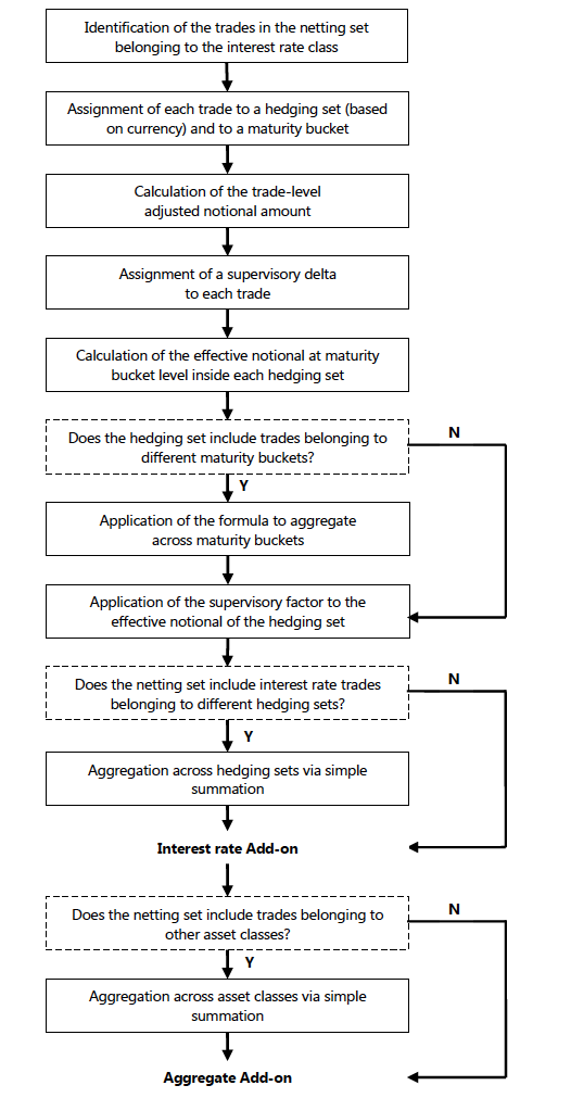
167. The add-on for interest rate derivatives is the sum of the add-ons for each hedging set of interest rates derivatives transacted with a counterparty in a netting set. The add-on for a hedging set of interest rate derivatives is calculated in two steps.
For a basis transaction hedging set, the supervisory factor applicable to its relevant asset class must be multiplied by 0.5.
FlowChart for IR add-on
And a summary of the steps given in the BCBS document.
Examples
Ordinarily I would now include a few worked examples for RC and PFE, however in the interests of time, will leave that to another day.
However for those of you interested, I would refer you to Annex 4a and 4b of the bcbs279 document.
Alternatively a Google search for “SA-CCR Calculator” will show a number of free calculators.
The End
Thats it for today.
SA-CCR is effective 1-Jan-2017.
It improves on existing non-IMM methodologies for Credit exposure.
Particularly for Cleared and Bi-lateral margined Derivatives.
The PFE AddOn component utilises Swap notionals.
Compression (triReduce, CCP or SEF) are effective methods to reduce the PFE AddOn.
Resulting in lower Credit Exposure and Capital.
I plan to cover this and other aspects in future articles.
UPDATE: We now offer free 14-day trials for our SA-CCR for Excel product
Excellent paper !
I FINALLY understood the SA CCR ! (BIS like the over complicated sentences)
It can be completed with the 4 examples in Annex of BCBS279