- Various risk charges must be calculated under the Standardised Approach of the FRTB.
- These risk charges are split into Delta, Vega and Curvature.
- Vega Risk Charge is complicated to calculate as we must build several co-variance matrices.
- We provide a step-by-step explanation of all of the calculations involved.
- We use Excel throughout to calculate and illustrate the various stages involved in calculating the FRTB Vega Risk Charge.
Fundamental Review of the Trading Book
I am going to dig deep into the calculations required to explain the FRTB Standardised Approach for option products. This first blog will tackle the Vega Risk charge. Whilst the commentary concentrates on Rates products, the methodology is extensible into all other asset classes.
Our reference document throughout is the BCBS January 2016 publication “Minimum Capital Requirements for Market Risk.” With a working (and recently updated) ISDA SIMM IM model in Excel, the similarities of the calculations are striking. It may also be beneficial to take a look at my first blog on FRTB Excel Calculations.
If you are interested in replicating the calculations yourself, I would take a look at ISDA SIMM in Excel for more detailed explanations of the Excel formulae.
1. Risk Inputs
We first find the sensitivity to each risk factor. This is the input to our FRTB model. For Vega Risk, these risk factors are defined by a volatility grid.
![]()
The “two dimensions” referred to are simply the maturities of both the option expiry and the underlying swap. Our inputs are therefore the following sensitivities:
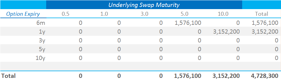
Showing;
- The expiry time of the option on the vertical axis
- The maturity of the underlying (in our case an IRS) along the horizontal axis
- The input sensitivity is the Vega multiplied by the implied volatility (see our ISDA SIMM – Swaptions blog).
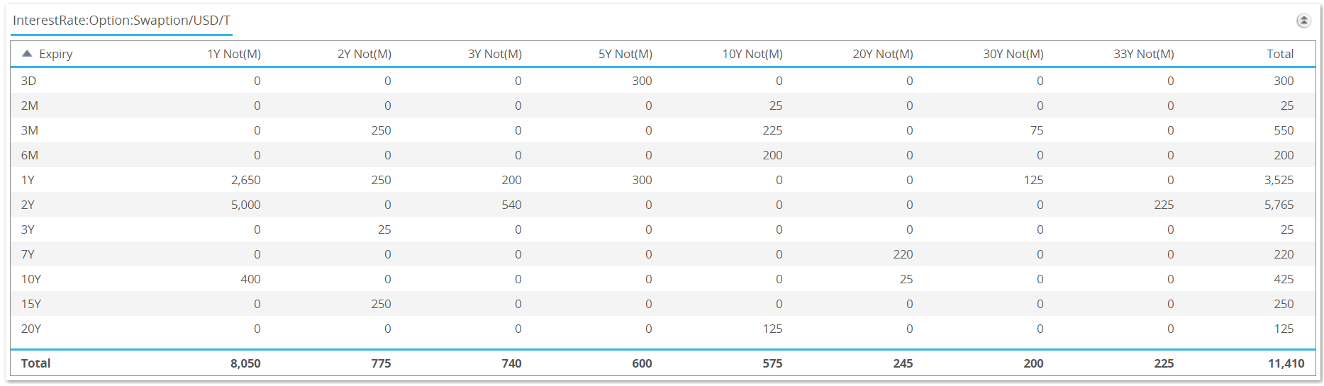
As a side note, whilst ISDA SIMM collapses this grid so that Vega is described along a single axis, FRTB approaches Vega risk in a different manner. This has implications for data manipulation down the line. FRTB is more akin to how we look at Swaption volumes in SDRView Pro:
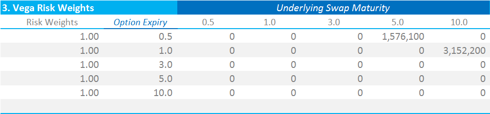
2. Risk Weightings
We now apply the appropriate risk weighting to the grid of Vega risks. The FRTB documentation defines the Risk Weighting as:
\( \tag {1} RW_{k} = min \big[ 0.55 \frac{\sqrt{60}}{\sqrt{10}}; 100 \% \big] \)Which in essence means that the Vega Risk Weight is a single point vector equal to 100% for Interest Rates. This is a particular quirk in the FRTB documentation. The \( \sqrt{60} \) is a variable by risk class, but there are only large cap equities that actually result in a risk weight less than 100%. It would have been easier just to say that…..hey ho.
My Vega Weighted Sensitivities that I need to carry forward now look…exactly the same as my input sensitivities! At least this bit is simple then.
3. Correlations (a.k.a “the fun part”)
Last week we had the joy of creating a new co-variance matrix to combine Delta IM amounts for a multiple currency portfolio in ISDA SIMM. Turns out, that was merely a warm up act for Vega Risk in FRTB.
For our grid of Vega Risks, we must now define the co-variance of each point with every other point. This is defined as:
\( \tag {2} ρ_{kl} = min \big[ ρ_{kl}^{(Expiry)}.ρ_{kl}^{(UnderlyingMaturity)}; 1 \big] \)
Meaning that we have to look at the maturity of both the option expiry and the swap itself to know what correlation factor to apply. This presents some nice spreadsheeting challenges in Excel!
The FRTB formula to calculate each \( ρ_{kl} \) looks fairly daunting:
\( \tag {3} ρ_{kl} = e^{-α.\frac {|T_{k}-T_{l}|}{min(T_{k};T_{l})} }\)In reality, α is equal to 1% and we are just multiplying it by the ratio of the maturity difference divided by the shortest maturity. Fairly simple….
The key thing is that we have to calculate \( ρ_{kl}\) for both the option expiries and the underlying swap maturities. That gives us a very large grid of co-variance.
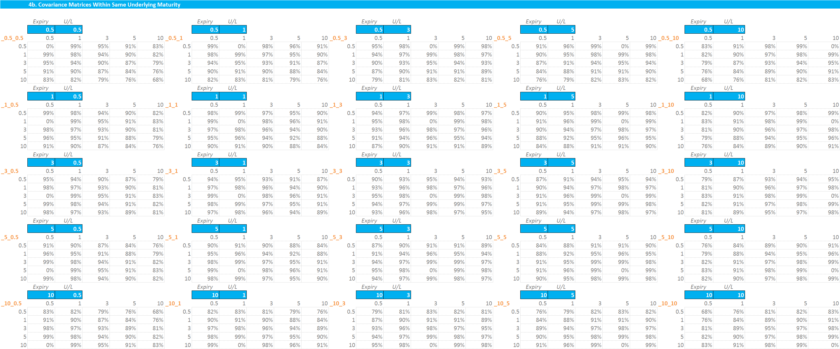
4. Calculate all Vega Correlations according to Equation (3)
This interim step gives us a very large co-variance matrix of expiries and underlying swap maturities:
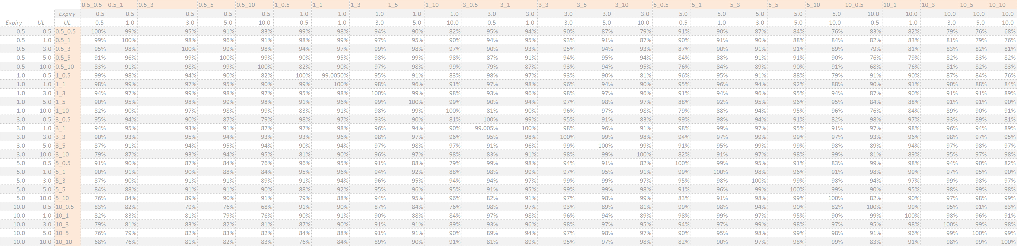
Showing;
- Every co-variance possible between all expiries and all underlyings.
- For example, a 1y into 10y has a co-variance of 99% (rounded) with a six month into ten-year.
- This co-variance is slightly lower if we look at a 1y into 10y with a six month into five-year (98% (rounded). This makes intuitive sense.
- The grid above depicts a 1y into 10y having 100% co-variance with another 1y into 10y. We’ll get into that later.
5. Vega Risk Charge
The aggregation formula that is used to calculate the Vega Risk Charge under FRTB is identical to the one used to calculate the Delta Risk Charge:
\( \tag {4} \large K_{b} = \sqrt{\sum\limits_{k}{WS_{k}^2+{\sum\limits_{k}}{\sum\limits_{(k)≠(l)}ρ_{kl}WS_{k}WS_{l}}}}\)Where;
\( {WS_{k}}\) is the Vega Sensitivity at a given tenor multiplied by the Vega risk weighting.
\({ρ_{k,l}}\) represents the correlation of the “WS” terms from one tenor (“risk vertex”) to the next. These correlations (co-variances) are the ones calculated in our large grid above.
This presents us with a challenge in Excel. How do we combine each cell in the below grid with the huge co-variance matrix?
x = ?
I broke this down into the following steps in Excel:
- Create a 5×5 co-variance matrix that applies to each point in our Vega Risk grid. This means 25 individual 5×5 co-variance matrices.
- For trades with the same underlying swap maturity AND expiry, I needed to include a co-variance of 0%, otherwise I double-counted that risk.
- For trades with the same expiry but different underlying swap maturity, I had to include a co-variance of 100% to include the risk.
- This results in 50 individual 5×5 co-variance matrices. There are two sets of 25, one with 100% and one with 0% for the matching expiry and underlying points.
What this says is:
- For a 1y into 10y Swaption, we have a known co-variance matrix with all other 24 points on the grid.
- These co-variances will be different for e.g. a 1y into 5y or a 6 month into 10y.
- By calling the relevant co-variance matrix into each point on the grid, I can simply calculate the sum product of the Vega Risks with that co-variance matrix.
This implementation in Excel may not be the most succinct way to do it, of that I am convinced. But it makes error-tracking and sanity checking fairly straightforward, as all of the calculations are very granular. Feel free to contact us if you have other suggestions on how to achieve the same.
6. Nearly Calculate the FRTB Vega Risk Charge
For our simple portfolio of two risk factors, we have the following calculation grid:
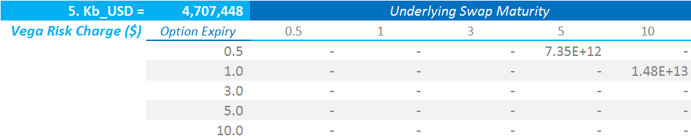
- It looks a little underwhelming at first pass.
- The implementation in Excel is the same as our “sumproducts” for ISDA SIMM. The only difference is that we must be clever in which covariance matrix that we reference (for those interested, I name the co-variance matrices by their vectors (e.g. “0.5_10” ) and use an “indirect” reference to this).
7. Run the Scenarios for Vega Risk Charge
Our final step is a familiar one. As we explored in our first FRTB calculations, the biggest difference to ISDA SIMM is that we must multiply our correlations (\( ρ_{kl}\) from above) by 0.75, 1.0 and 1.25 before we find out the final Risk Charge. In the case of Vega Risk, this means that we must multiply the large co-variance matrix (and all of its’ 50 child matrices) by 0.75, 1.0 and 1.25. The ultimate Risk Charge is the largest of the three results.
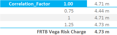
This takes us to the end of today’s calculations. Our original FRTB blog shows how to perform the same calculations across multiple currencies.
In Summary
- We show how to calculate the FRTB Vega Risk Charge under the Standardised Approach.
- This will have to be calculated for all options portfolios on a daily basis.
- The calculations present some implementation challenges and represent the most complex scenarios we have yet encountered via our blogs on FRTB and ISDA SIMM.
- There are a large number of co-variance matrices that must be derived.
- We provide example Excel implementations of how these calculations can be achieved.