ISDA SIMM™ in Excel – Equity Options

• We build an IM calculator in Excel for Equity Options under ISDA SIMM™.
• The methodology builds on the margin methodology for Swaptions, and uses very similar formulae.
• We cover all forms of IM. This blog is for the Vega and Curvature Margin.
• There are subtle differences to the implementation for Rates.
• UPDATE: We now offer free 14-day trials for our SIMM for Excel product

Equity Options Initial Margin

So far we have successfully built and maintained Excel spreadsheets to calculate Delta IM for rates products, for multi-currency portfolios and also for Swaptions that cover both Vega and Curvature IM. With the remit of ISDA SIMM™ to be easy to replicate, this week it is the turn of Equity Options. The ISDA reference docs are here.

1. Risk Sensitivities For Vega and Curvature

The input for ISDA SIMM at each maturity is volatility multiplied by vega. We need to know what type of vol and the units of measurement, so we should be a little bit more explicit here:

\( \tag {1} VR  =  \sum σ \frac{dV}{dσ}\)

Where;

VR = The Vega Risk input required for ISDA SIMM of each security.

σ = The volatility at each tenor. The tenors are the same as used for Swaps.

\(\frac {dV}{dσ}\) = change in price with a change in vol, commonly referred to as “vega”.

In a departure to how we treat Vega risk for Interest Rates, we take the Vega as the input for Equity options, and calculate the volatility according to the below equation:

\( \tag {2} σ_{kj} =  \frac{RW_{k}\sqrt{365/14}}{φ^{-1} (99\%)}\)

Meaning that we need to multiply the Vega input by the Risk Weight (of the underlying Delta), multiplied by “SQRT(365/14)/(NORMSINV(0.99))” in Excel equation-form. This means that there is no link between the Vega Risk Weight and the maturity of the option. This is, instead, dealt with via Curvature Risk (see below).

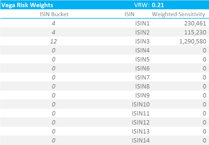
2. Risk Weightings

We now apply the requisite Vega Risk weight to each bucket, according to the ISDA calibration. This is a single weight of 0.21.

For now, I will run these calculations assuming that we are below the Concentration Threshold. Please refer to my separate blog on Concentration Thresholds for the implementation of these risk multipliers.

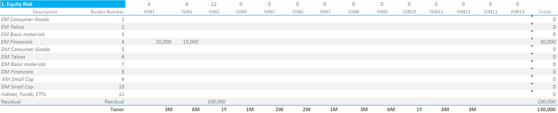
For our simple portfolio, this shows that;

• We are able to simply sum all Vega Exposures across tenors but belonging to the same ISIN together. No co-variance/correlation factors to deal with.
• Multiple ISINs can be mapped to the same Risk Bucket (e.g. ISIN1 and ISIN2 both belong to Risk Bucket number 4).
• These figures are our “Weighted Sensitivities” (“WS terms”) that can then be carried forward into the more meaty calculations below.

3. Correlations

Staying with Vega Risk, we must now aggregate both within and across Risk Buckets. Please refer to our blog on Equity Derivatives to see the differences with Rates products that this implies.

We are able to use exactly the same methodologies as used for Equity Delta when calculating the Vega Risk Margin for this portfolio. We therefore have the following two co-variance matrices to deal with:

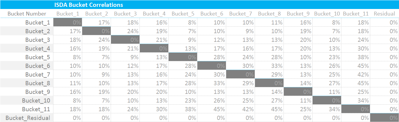
We use the correlations on the left (in yellow) to calculate Kb per Risk Bucket and use the correlation matrix on the right to combine the Kb and Sb values per Risk Bucket to arrive at an overall Vega Risk Margin. These calculations were covered in-depth in the previous blog – and for ease of reference are reproduced below:

This is how I implement the key formula that we keep on revisiting in these blogs:

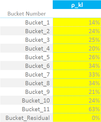
\( \tag {3} K = \sqrt{\sum\limits_{k}{WS_{k}^2+{\sum\limits_{k}}{\sum\limits_{l≠k}{f_{kl}{ρ_{kl}}{WS_{k}}{WS_{l}}}}}}\)

Where;

\( {WS_{k}}\) is the input Vega multiplied  by the volatility and the ISDA-supplied risk weighting, as per step 2.

\({f_{kl}}\) is the modification we have to make to our correlations in the case that one of the risk factors is above the Concentration Threshold. See my blog on this for more. For now, we assume we are below the CTs.

\({ρ_{kl}}\) is a correlation matrix. It defines the correlation of the “WS” terms from one ISIN to the next (i.e. between k and l in the nomenclature). So for example, ISDA deem that ISINs falling within Bucket 4 have a correlation of 20% with each other. These are not currency dependent – one table serves all currencies.

I therefore calculate the value of “K” for each bucket, squaring the WS terms and adding in the sumproduct of correlation x WS. We then calculate the value of Sb;

\( \tag {4}{S_{b} = max(min({\sum\limits_{k}}WS_{k},K_{b}),-K_{b})}\)

\( {S_{b}}\) is either the sum of all of the “Weighted Sensitivities” or the value of K for bucket b. We first take the smaller of the sum of the WS’s and then the larger of this and  “negative K” for bucket b. This means that \( {S_{b}}\) can, in some instances, be a negative number.

The calculation grid shows it more succinctly than I can put it into words:

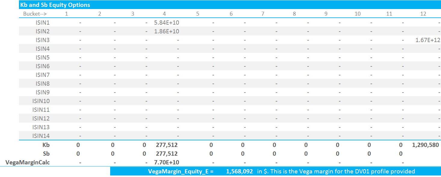
Showing;

• As per Equity Deltas, we use the Sb values combined with the covariance matrix for cross-bucket exposures to aggregate Vega amounts for Buckets 1 through to 11.
• Bucket 12, the Residual Bucket, carries an uncorrelated weighting, equal to the value of Kb for Bucket 12.
• For our portfolio, we see a Vega Margin amount of $1,568,092.

4. Curvature Risk

Our canny readers will have noticed that the above does not cater for Gamma or Theta. For the ISDA SIMM model, we instead calculate Curvature Risk. This is where the time to maturity of our Equity Options comes into play. The calculations are almost identical to the ones we performed for Swaptions.

First, we calculate the Curvature Risk:

\( \tag {5} CVR_{ik}  =  \sum\limits_{j} SF(t_{kj}) σ_{kj} \frac{dV_{i}}{dσ}\)

Where;

\( SF(t_{kj}) \) is a scaling function associated with the time to expiry of the option. At each tenor, SF is simply equal to:

SF = 0.5 * minimum(1, 14/(maturity in days))

We can therefore simply multiply our previous Vega Risk Weights grid by the value of SF for each option expiry;

To then combine these Curvature Risk Weights into a single Curvature Risk Margin, we must first square the correlations used for Vega Risks:

And then we have to calculate two new terms, θ and λ;

\( λ = (2.58^2 -1)(1+θ) – θ, \)

where;

\( \tag {6} θ = \frac{\sum\limits_{b,k}CVR_{b,k}}{\sum\limits_{b,k}|CVR_{b,k}|}\)

Equation (6) is capped at zero. We must calculate 2 values of θ and λ  – one for buckets 1-11 for the non-Residual risks, and the same for the Residual bucket.

Both θ and λ are trivial to calculate once you are familiar with the terminology. Here are a couple of pointers:

1. The “2.58” is a placeholder for the Excel formula “NORMSINV(0.995)”. This is the 99.5th percentile of the standard normal distribution.
2. You must calculate θ and λ across Buckets 1-11, and then across the Residual Bucket as independent values.
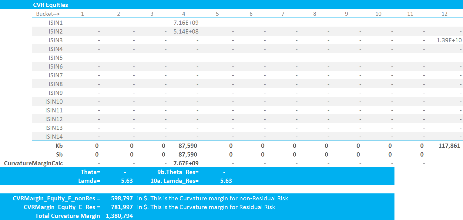
3. Both values of θ are equal to zero for our portfolio (which is pretty common for simple portfolios).
4. Both values of λ are 5.6348966.

Our final two steps are to calculate the Curvature Risk Margin for non-Residual and Residual buckets. For non-residual buckets, we use the following formula:

\( \tag {7} Curvature Margin = \sum\limits_{b,k}{CVR_{b,k}+λ\sqrt{\sum\limits_{b}{K_{b}^2+{\sum\limits_{b}}{\sum\limits_{(c)≠(b)}{γ_{bc}^2}{S_{b}}{S_{c}}}}}}\)

with the above term floored at zero. Remember that \({γ_{bc}^2}\) is the correlation matrix on the far right in our previous screenshot. For our portfolio, the Curvature Margin for non-Residual buckets is $598,797.

And for the Residual Bucket, this same equation reduces down to the simple form:

A nice and simple formula to finish on! The total Curvature Margin is the sum of non-Residual and Residual Curvature Margin. For our portfolio, the Curvature Margin for the Residual bucket is $781,997. Again, the calculation grid below summarises this better than the five preceding paragraphs:

In Summary

• ISDA SIMM Margin for Equity Options can be calculated in Excel.
• We must first calculate the Vega Risk Margin.
• And then calculate the Curvature Risk Margin.
• The total ISDA SIMM Margin is the sum of Vega Risk and Curvature Risk Margins.
• The biggest difference with Rates calculations is that one of the risk buckets, the so-called residual bucket, is treated as an independent risk with no correlation to other risk buckets.
• We hope you have found this walk-through informative. For those trying to replicate, please don’t hesitate to contact us.